

One of the ways we can simplify and reduce the size and computational complexity of a finite element model is by taking advantage of any symmetries it may have. Paring down models is particularly important when we are dealing with computationally heavy wave electromagnetics projects. However, due to their vector nature, electric and magnetic fields do not necessarily follow all possible symmetries geometry-wise. Therefore, special care and proof of correct implementation are always needed to retain consistency.
In this blog post, we will present the typical workflow in COMSOL Multiphysics®for exploiting symmetries in RF and wave optics modeling. We will focus on the widely usedElectromagnetic Waves, Frequency Domaininterface and cover the proper choice of boundary conditions, discuss how to effectively organize a model to validate obtained results, and take a look at various techniques for analyzing results, including far-field calculations and lumped parameter evaluations.
An Example of the Benefits of Applying Symmetry Conditions: A Plane Wave Scattering off a Nanosphere
Let’s start with a basic wave optics example of a plane wave scattering off a nanosphere suspended in free space. Specifically, we will consider a plane wave of wavelength 500 nm polarized in thezdirection and propagating in the global positivexdirection and a nanoparticle of radius 100 nm with a complex-valued refractive index taken from the Optical material library (Rakic et al. 1998).
To model this scenario, we will use theElectromagnetic Waves, Frequency Domaininterface with theScattered fieldformulation and finish the surrounding free-space domain with perfectly matched layers to ensure there is no reflection on the exterior boundaries. For the outputs, among others, we are interested in the far-field scattering pattern. Therefore, we will add aFar-Field Domainfeature to obtain the corresponding visualization. We will use the defaultPhysics-controlled meshwith theResolve wave in lossy mediacheckbox active and aWavelength Domainstudy. A look at the COMSOL Multiphysics®UI highlighting some of these settings is shown below.
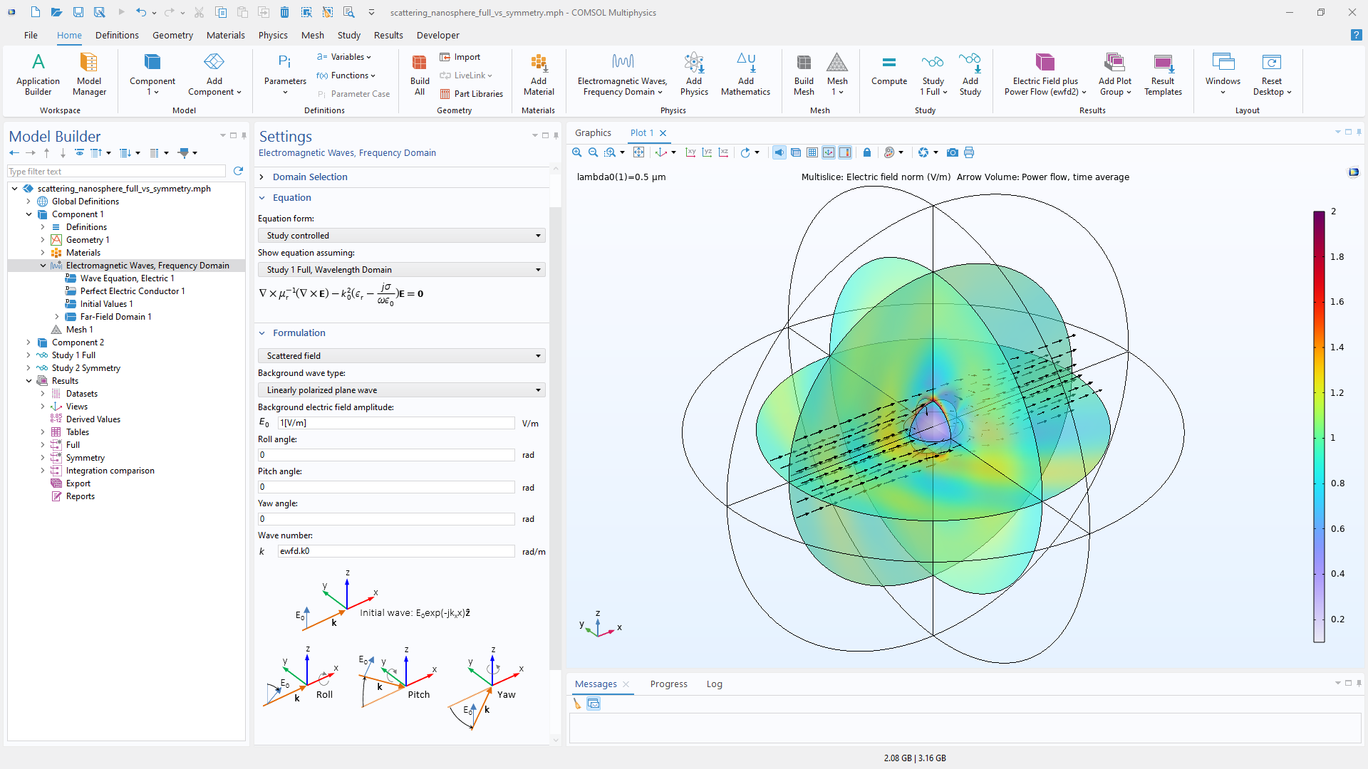 The full geometry model of a plane wave scattering off a nanosphere. TheScattered fieldformulation is highlighted in theSettingswindow. In theGraphicswindow, the resulting total field is shown (theMultisliceplot) along with the power flow in the system (theArrow Volumeplot).
While this example is rather modest in terms of the amount of memory and time required to obtain results, it never hurts to reduce these numbers. The more complex a model is or the more tests we need to run, the more significant of a performance boost we can get if we’re able to reduce the number of degrees of freedom (DOFs) involved. Exploiting symmetry is one of the most obvious and efficient ways to do so.
Note: Later in this post, we will discuss the performance boost for amodel of a patch antenna.
In terms of the geometry, given that the nanoparticle center is aligned with the origin, we have three possible symmetry planes: xy, zy, and yz. Let’s determine whether any of them are okay to use for reduction. Before we proceed, it’s important to discuss the behavior of electric and magnetic fields across a symmetry plane, along with the relevant governing equations.
Physics and Implementation of the Electromagnetic Field Symmetry
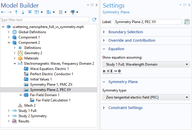
According to the properties of Maxwell’s equations, we can implement a plane of symmetry if we have either zero tangential electric fields or zero tangential magnetic fields across it. If there are zero tangential electric fields, we have mirror symmetry in the magnetic field; this can be described as\textbf{n} \times \textbf{E} = 0. If there are zero tangential magnetic fields, we have mirror symmetry in the electric field; this can be described as\textbf{n} \times \textbf{H} = 0.
The good news is that these mirror symmetries can be easily implemented in COMSOL Multiphysics®. As of version 6.1, theElectromagnetic Waves, Frequency Domainhas a dedicatedSymmetry Planecondition with options to choose between aZero tangential electric field (PEC)— equivalent to the basicPerfect Electric Conductorcondition — and aZero tangential magnetic field (PMC)— equivalent to thePerfect Magnetic Conductorcondition. Both cases are schematically illustrated below.
Note: Similar functionality is available in the AC/DC Module for the interfaces designed to handle electric andmagnetic fields.
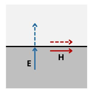
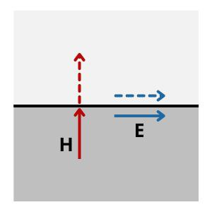
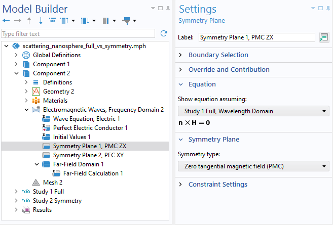
Two sketches illustrating two possibleSymmetry Planeconditions. The left image shows a mirror symmetry for the magnetic field, which is modeled with theZero tangential electric field (PEC)option. The right image shows a mirror symmetry for the electric field, which is modeled with theZero tangential magnetic field (PMC)option.
Keeping this information in mind, let’s return to our example and sort out where we can apply theSymmetry Planecondition.
Determining Possible Symmetries
The following is a rough checklist of questions to ask to streamline the selection of appropriate symmetry planes:
- Does the direction of wave propagation and scattering on a given plane allow symmetry to be exploited?
- What happens to the wave polarization in a possible symmetry plane?
- Can we consider either the tangential electric or tangential magnetic fields to be zero on a given plane?
- On the contrary, do we expect the orientation of these fields to change in space along the given plane due to a complex (e.g., circular) wave polarization?
- Do we expect the excitation of any higher-order modes that have a different symmetry?
How to answer these questions depends on the situation. Sometimes, an answer is straightforward. For instance, for our test case, we can immediately eliminate the yz-plane from consideration: The background field propagates toward it, and the scattering back and forth is expected to be different both with respect to the direction and amplitude.
Determining whether the other two planes can be used may require some reasoning and/or preliminary tests. The background field is polarized in the z direction so that we can consider the mirror symmetry for the electric fields (“E-fields”) in the zx-plane and the mirror symmetry for the magnetic fields (“H-fields”) in the xy-plane. The Mie scattering in this case doesn’t affect polarization in these planes and does not lead to generation of the modes that break the selected symmetry. Since we have a solution for the full geometry, we can easily confirm it by plotting a vector representation of the electric and magnetic fields in the zx and xy cut planes. This can be implemented with theArrow Volumeplot type, which is extremely handy when analyzing any vector fields.
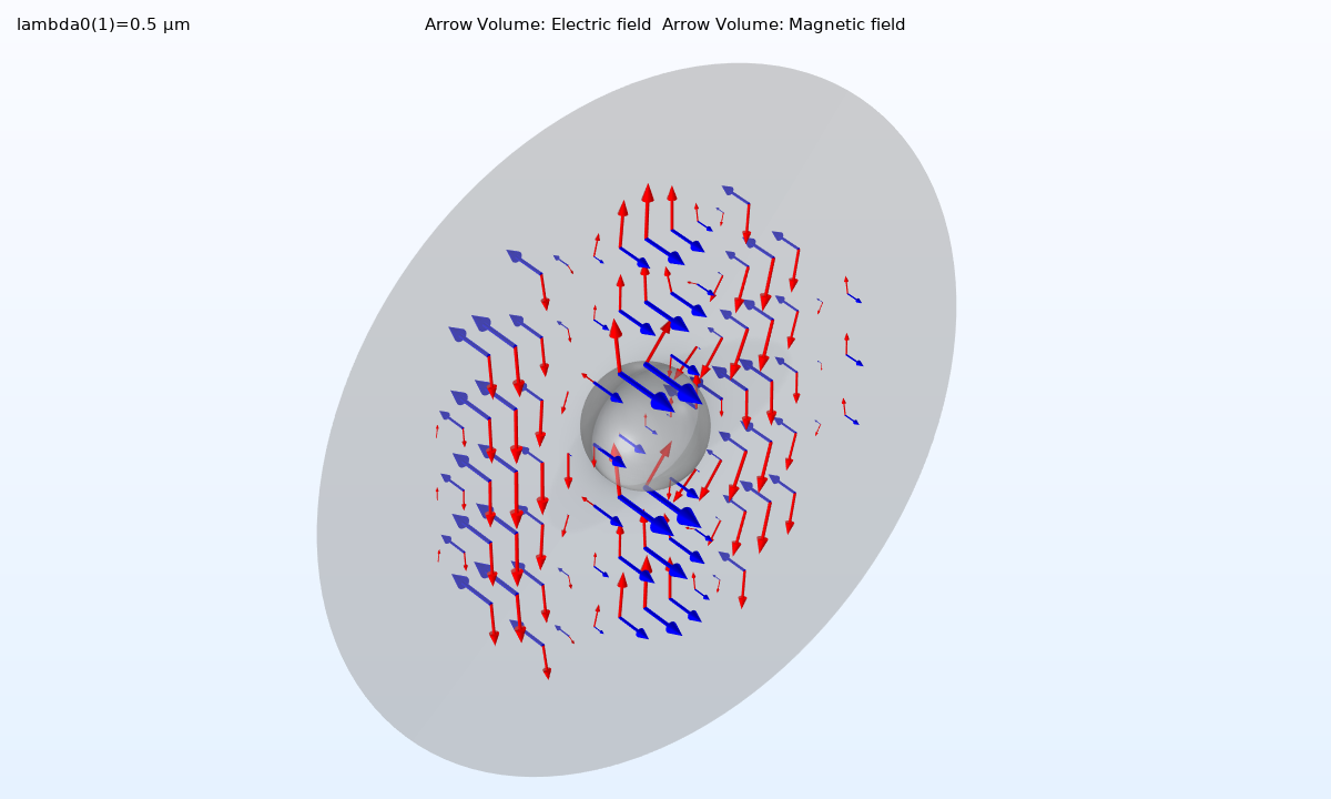
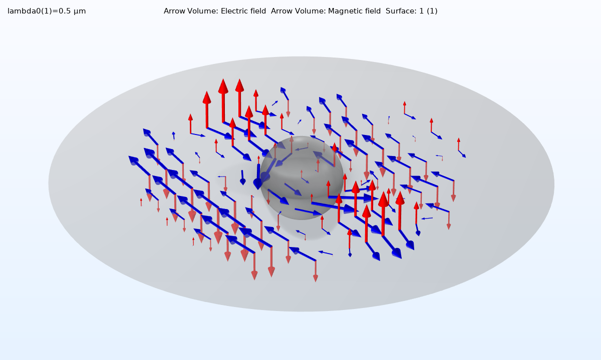
E-fields (red arrows) and H-fields (blue arrows) in the zy (left image) and xy (right image) cut planes.
TheArrow Volumeplots confirm that theSymmetry Planecondition can be applied to the zx-plane using theZero tangential magnetic field (PMC)option and in the xy-plane using theZero tangential electric field (PEC)option.
Now, it is time to exploit these simplifications in our model.
Implementing Symmetries in the Geometry and Physics
At the geometry level, we should create aWork Planefor every symmetry plane, use it to partition the whole geometry via aPartition Objectsoperation, and finally, delete any entities that are no longer needed using theDelete Entitiesoperation. This workflow is covered in detailhere. In our case, with the full model in hand, it makes sense to copy-paste the wholeComponent, which is the equivalent of duplicating it, and implement all of these geometry modifications in the secondComponent.
At the physics level, after we have reduced the geometry, the main change we need is to add theSymmetry Planecondition for every separate plane. It is preferable to use the Symmetry Plane condition instead of separatePerfect Electric ConductorandPerfect Magnetic Conductorconditions; when theSymmetry Planecondition is added, certain expressions are automatically adjusted in thePort,Lumped Port,Cross Section Calculation, andFar-Field Domainnodes. This last node is very handy for our example since evaluating the far-field results is of great importance here.
Note: You can use theGroup by continuous tangentoption in theGraphicswindow to select all of the required boundaries in one click.
Once we are done with the physics settings, we can add a newWavelength Domainstudy for the secondElectromagnetic Waves, Frequency Domaininterface and launch it. This brings us to the most interesting part of any simulation — visualizing and evaluating the results.
Analyzing a Reduced Model with Symmetry Conditions Assigned
As you can see in the screenshot below, the far-field visualization doesn’t require any extra settings to generate the full radiation patterns when we use theSymmetry Planefeatures and select theFrom Symmetry plane(s)option in the settings of theFar-Field Calculationsubnode.
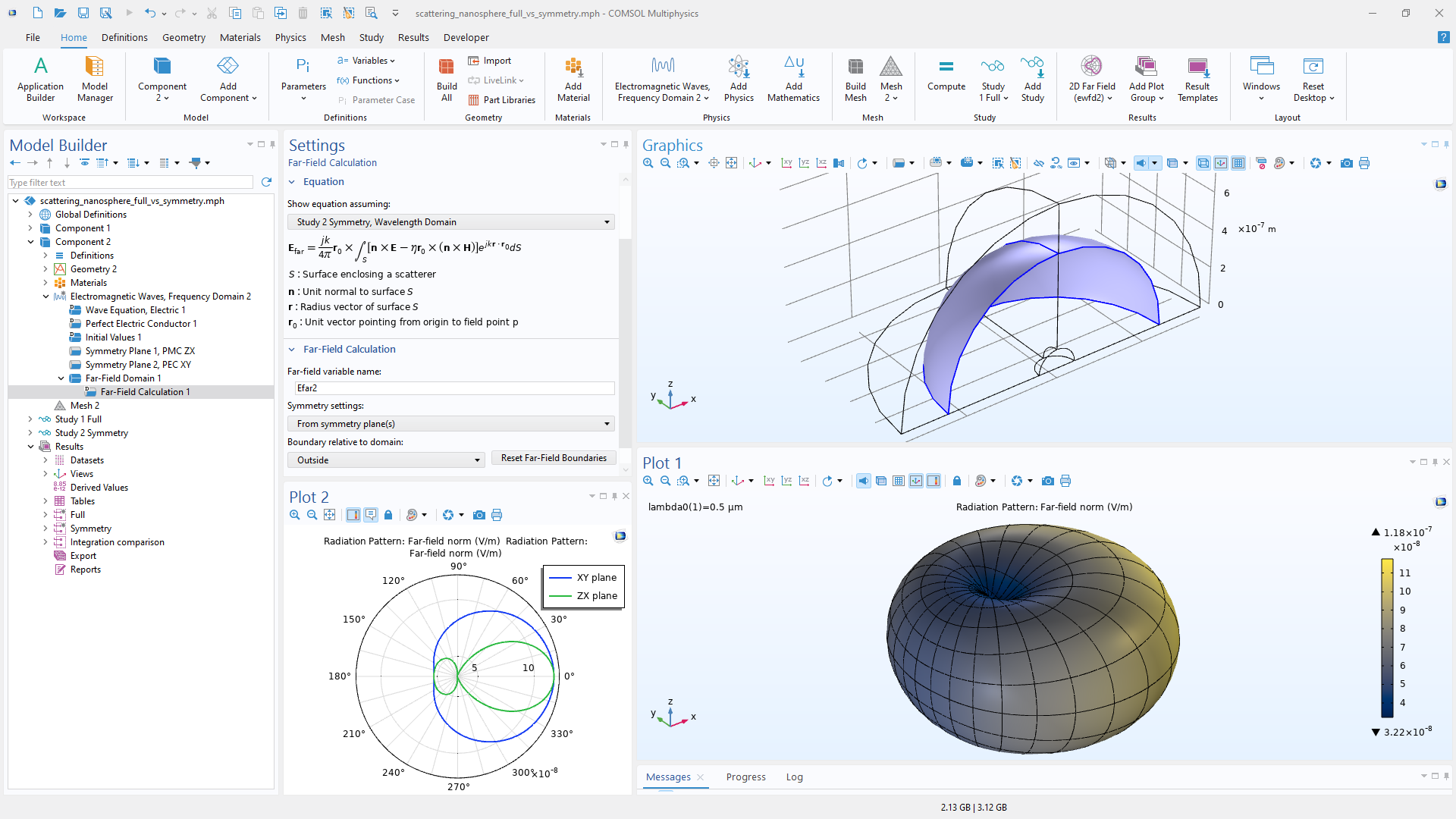 The reduced model of a plane wave scattering off a nanosphere with the two symmetry planes implemented. The far-field plots are shown. They automatically generate the radiation pattern for the full geometry.
The standard E-field plots, on the other hand, are shown using the reduced geometry by default. However, you can add several extraMirror 3Ddatasets to restore the full geometry when visualizing results. These datasets have the advanced settingVector transformation, which needs to be aligned with the symmetry implemented. In our example, for the zx mirroring, we need theAntisymmetricoption. A heads-up: TheAntisymmetricoption is only required if you are going to plot vector fields; for the scalar variables, it is best to keep the default settings.
The same consideration holds when we perform any integration operation, such as estimating the total power absorbed in the lossy particle; we can either use an extraMirror 3Ddataset or simply add the corresponding multiplication factor manually when using the defaultSolutiondataset.
Two More Examples
Let’s take a look at two more examples where we can exploit symmetries. We’ll go through them a bit faster, focusing only on the aspects that we couldn’t demonstrate with the nanosphere scattering model. These two examples, as well as the first model, areavailable for downloadat the end of this blog post.
A Patch Antenna Case with Lumped Port Modeling
Antenna modeling is another area where we can benefit from exploiting symmetry. To demonstrate, we will consider theMicrostrip Patch Antennatutorial model from COMSOL’s open-access Application Gallery. We will show how partitioning it in the yz-plane and implementing aSymmetry Planecondition with theZero tangential magnetic field (PMC)option affects both the plotting of the lumped parameters and the general performance of a regular frequency sweep.
The core consideration here is that, when we reduce the model, we are cutting the radiating Lumped Port in half. This condition comes with the option to perform aCharacteristic impedance adjustment by symmetry plane. Selecting this checkbox means we can keep theCharacteristic impedancevalue of the full geometry even when we have decreased the port’s area by a factor of two, giving us an opportunity to directly evaluate all variables that depend on this value, such as the lumped port voltage, S-parameters, realized gain, etc. However, once the lumped port power and impedance have been calculated under the hood by the boundary-based integration, we need to scale them to get the correct values. This scaling requirement is similar to the one we saw for the volumetric loss integration in the first example.
Another thing that we should pay attention to is the direction in which we cut theLumped Portboundary and how this affects the input voltage amplitude. For the patch antenna model, the thickness remains the same, so there is no need to scale the voltage amplitude. However, if the symmetry were cut perpendicular to the electric field direction across theLumped Port, we would want to scale the voltage amplitude by adding the corresponding multiplier to the reduced model. The same considerations hold when defining power within theLumped Port, as the conversion, in the form ofV0 = \sqrt {2 \cdot P0 \cdot Z0}, is applied automatically.
Evaluating the Results
When we compare all of these results with the full geometry reference, there may be a notable difference. While this can seem confusing initially, it is just an indication that a mesh refinement study is needed. In other words, for the reduced model, we see better resolution of the lumped port, which is important because it increases the accuracy of the lumped parameters calculated. The same may be true for other small geometry details. One way to implement sufficient refinement here is to select theRefine conductive edgesoption for the mesh in both the reduced and reference versions. The next screenshot demonstrates the final results. By putting some time and effort into further investigation, you can get even better correlation between the reduced and full model.
Note: Another way to find an optimal mesh distribution is by running aFrequency Domain, RF Adaptive Meshstudy. View details in thecorresponding tutorial model.
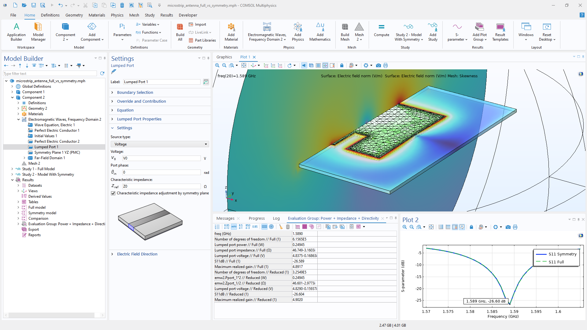 The Microstrip Patch Antenna model using theSymmetry Planecondition. In Plot 1 (top), you can see the optimized mesh configuration generated by theRefine conductive edgesfeature, along with the E-field pattern shown in a logarithmic scale. Below Plot 1, the table of selected lumped parameters (left) and the plotted S11 resonance curves (right) both show strong correlation between the full and reduced model.
A positive side effect of implementing symmetry in this case was that it brought us better accuracy, but how did it affect the computation? The table below shows the results of two test runs, comparing the performance of the full model with the reduced model in terms of the number of DOFs, the RAM used, and the solution time. In a nutshell, halving the model takes 42% less time to solve and uses 25% less memory. These numbers will be hardware dependent, and more resource-demanding projects will yield even better performance boosts.
| Criteria | Full Model | Model with Symmetry | Reduction |
|---|---|---|---|
| Number of DOFs | 615,646 | 325,490 | 47% |
| Physical RAM used | 5.4 GB | 4.05 GB | 25% |
| Solution time (36 frequency points) | 180 s | 108 s | 42% |
Performance comparison based on the modified Microstrip Patch Antenna model. Both the RAM used and solution-time metrics were reduced by 25% and 42%, respectively.
A Rectangular Waveguide and the Higher-Order Modes
Calculations that involve consideration of several different modes in a system also require careful attention when implementingSymmetry Planeconditions. Such a project may directly involve an eigenvalue calculation or may be a frequency-domain model featuring excitation of various modes within a simulation domain or via a set ofPortconditions.
As an example, let’s take a look at a simpleMode Analysisstudy of a rectangular waveguide cross section and focus on the effect of leveraging a vertically cut symmetry. When we initially examine the modes of interest, we find that, among the first six, TE10, TE11, and TM11 follow the perfect magnetic conductor (PMC)-type symmetry with respect to the vertical cut, whereas TE01, TE20, and TE21 have the perfect electric conductor (PEC)-type symmetry. That said, if we were to consider a multimode waveguide with both TE10 and TE20 modes present, we would need to retain the full geometry; otherwise, we would lose one of the modes and therefore get incorrect final results.
A good practice for every complex multimode project is to preliminarily investigate the modes of interest in the system, as we did here. For a waveguide model, performing the extendedMode Analysismakes sense. For a general case, some common-sense reasoning or anEigenfrequencycalculation can be handy.
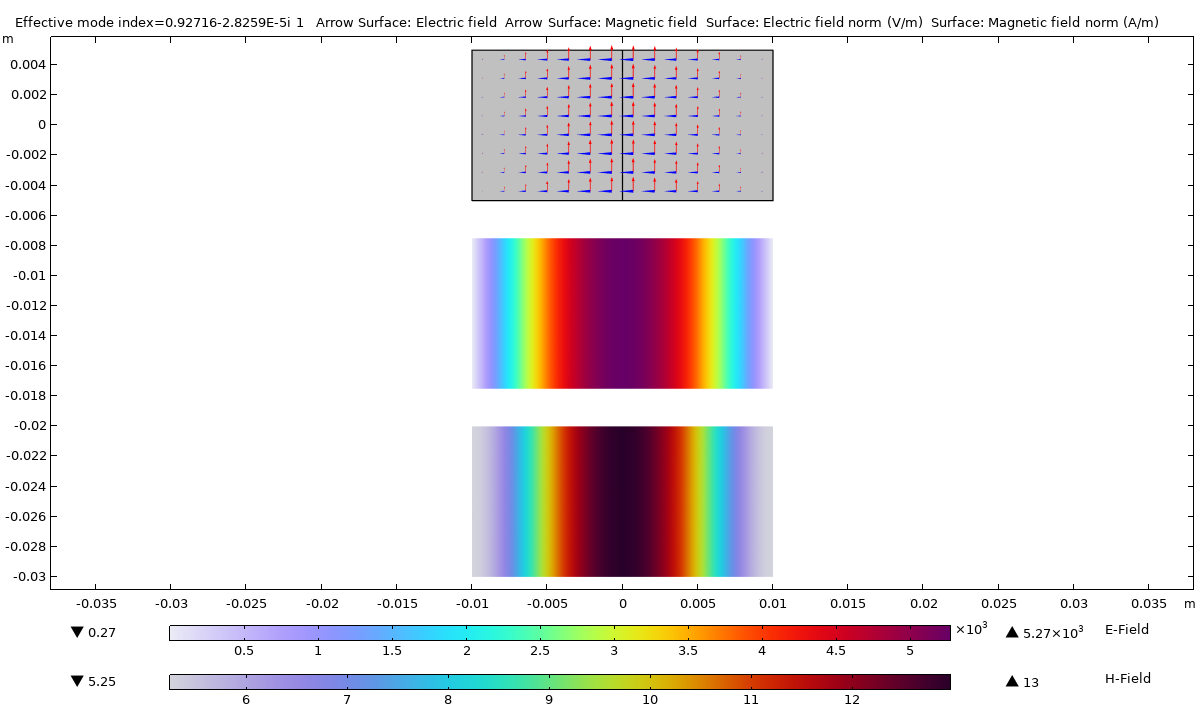
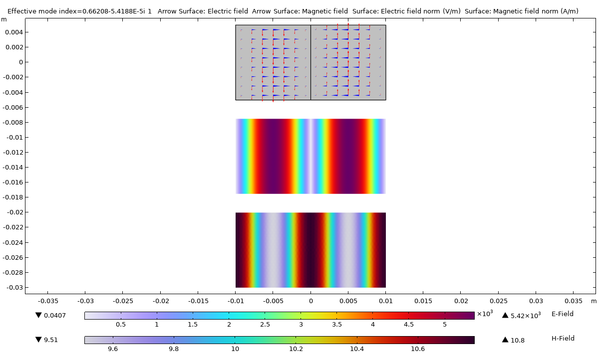
TE10 (left image) and TE20 (right image) modes of a rectangular waveguide. In the top plot for both modes, the tangential E-field is marked with red arrows and the H-field is marked with blue arrows. The middle plots show the magnitudes of the E-field and H-field distributions. If symmetry were exploited, the TE10 mode would require the PMC condition with respect to the vertical cut, while the TE20 mode would need the PEC condition.
Two additional modifications should be kept in mind for certain cases: If we rely on an approach that picks a mode based on its sequential number, this approach needs to be updated accordingly when we reduce the model via symmetry. If we have aPortcondition, we should rememberto scale thePortinput powerand reduce it proportionally to its surface decrease.
Final Reflections on Symmetry Plane Conditions
In this blog post, we demonstrated how to exploit symmetry conditions in theElectromagnetic Waves, Frequency Domaininterface following some simple rules and utilizing theSymmetry Planecondition. When properly used, this approach enables better computational performance for various types of scattering, radiating, and waveguiding problems — with even more accurate results. While they are almost fully automated, some operations like volumetric or boundary integrations may require extra scaling when you are visualizing and evaluating the results. When implementing a reduced model, we encourage everyone to run a preliminary simplified model first and compare it with the full configuration to ensure consistency.
Try It Yourself
Try implement symmetries in the tutorial models we discussed in this post and check out all the supplementary settings and various options for visualizing and evaluating your results.

Comments (0)