学习中心

Course:

Modeling Magnetohydrodynamic Flow

Setting Up the Electromagnetics Interface

In the previous part of this course, we discussed the process of starting to build a magnetohydrodynamics (MHD) model in COMSOL Multiphysics^®by adding the required geometry, materials, physics interfaces, andMagnetohydrodynamicscoupling. Over the next two parts of the course, we will discuss how to set up interfaces with the required domain and boundary conditions for MHD modeling. Here, we will focus on setting up theMagnetic FieldsorMagnetic and Electric Fieldsinterface for solving the electromagnetic side of the problem. We will go over defining materials as solids or fluids, applying uniform magnetic background fields, and handling different conductivities of walls containing fluid. Setting up the fluid flow interface will be covered in Part 5 of this course.

The Magnetic Fields Interface

When theMagnetic Fieldsinterface is added to an MHD model via theMagnetohydrodynamicscoupling, the default external boundary conditionMagnetic Insulationand theFree SpaceandAmpère's Law in Fluidsnodes are added. These features define the equations that are being solved for.

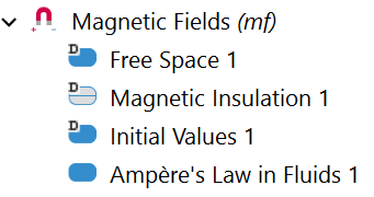
A Magnetic Fields node and the Free Space, Magnetic Insulation, and Initial Values subnodes.
TheMagnetic Fieldsnode and the default subnodes.

Defining Free Space, Solids, and Fluids

TheMagnetic Fieldsinterface includes three formulations of the equations for Ampère's law that are designed to be used in different materials:

Free Space, which is designed to handle Ampère's law in air, which has a conductivity very close to zero. It applies stabilization techniques to handle this very low conductivity
Ampère's Law in Fluids, which is designed to handle fields in liquid materials that can move without their external boundaries moving
Ampère's Law in Solids, which handles fields in solid materials where motion involves a deformation of the mesh due to the deformation or translation of the structure

TheFree Spacefeature is normally the default feature defining the equation that is solved in all domains, withAmpère's Law in SolidsandAmpère's Law in Fluidsnodes added to override it in solid and fluid domains. However, by selecting theMagnetohydrodynamicsinterface, an initialAmpère's Law in Fluidsfeature is added and applied to all domains, as theMagnetohydrodynamicscoupling is only valid in domains selected in anAmpère's Law in Fluidsfeature.

The first step in setting up theMagnetic Fieldsinterface is removing any nonfluid domains from theAmpère's Law in Fluidsselection and adding anAmpère's Law in Solidsnode that is assigned to solid domains.

The Ampère's Law in Fluids Settings window in COMSOL Multiphysics. A magnetohydrodynamics pump model using theFree Space, Ampère's Law in Fluids, andAmpère's Law in Solids features to define Ampère's law in the air, fluid, and solid regions.

Field Components Solved For Feature

TheMagnetic Fieldsinterface can only be used in either 2D or 2D axisymmetric models for magnetohydrodynamics modeling. In these formulations, there is a choice of how many components ofshould be solved for — its in-plane components, its out-of-plane components, or the full vector of three components. Any nonsolved components ofare set to zero. The directions the current can flow is determined by the nonzero entries of. Because of this, since only out-of-plane currents are allowed for MHD models using theMagnetic Fieldsformulation, only the out-of-plane option is allowed for theField components solved forsetting when creating MHD models. This selection generates an in-plane magnetic field.

The Out-of-plane vector potential option in the Magnetic Fields Settings window. Only theOut-of-plane vector potential option can be used in theField components solved for setting to preserve the assumption that the induced current is out of plane.

Defining Uniform Background Fields

A common feature of MHD models is the presence of a uniform background magnetic flux density, which is the source for the magnetohydrodynamic motion. This uniform background field can be applied in theMagnetic Fieldsinterface by using theReduced Fieldformulation in the settings for theBackground Field in the Magnetic Fieldsnode.

TheReduced Fieldformulation specifies that the total magnetic vector potential in the model can be written as the sum of a potentialfor a known background fieldand a component that is solved for, known as the reduced potential, that relates to a reduced field. The total field can then be calculated as.

In a linear model, this simplifies to the idea that a solution for the field can be decomposed into a linear supposition of component fields — the background field and the reduced field.

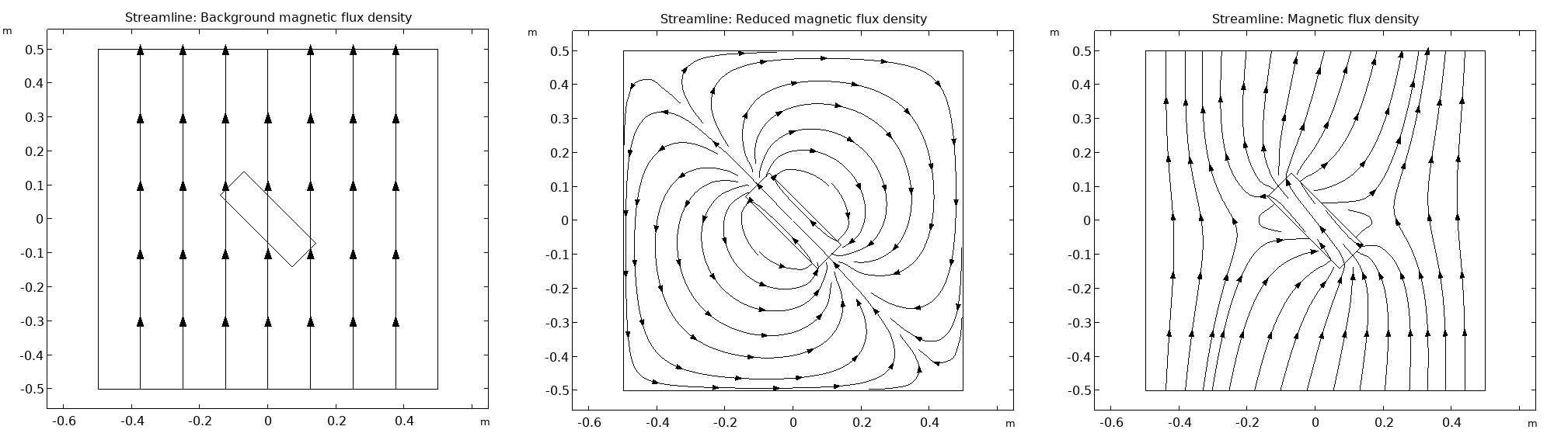Three 2D plots of the background, reduced, and total magnetic flux density. Demonstrating the reduced field formulation. A bar magnet is placed inside a uniform background field, and the total field is solved for using the reduced field formulation. The background magnetic flux density (left); the reduced field (middle), which consists of the field from the magnet, plus any corrections that need to be added to the background field for the total field to satisfy the boundary conditions; and the resulting total magnetic flux density (right).

By choosing theReduced Fieldformulation option in theMagnetic Fieldsinterface, it is possible to specify the background field by either specifying the magnetic vector potential or by specifying a uniform magnetic flux density in the model. This allows the uniform background flux density to be directly inserted.

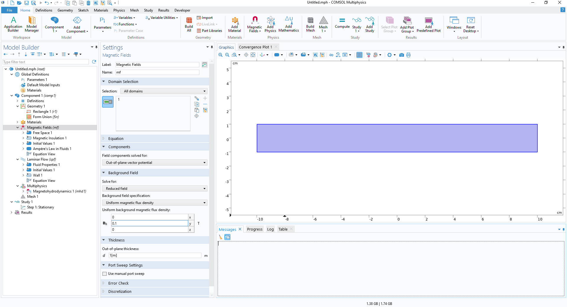The Magnetic Fields Settings window with the background field options being configured. Defining a uniform background field using theReduced Field formulation.

When working with theReduced Fieldformulation, it is recommended to use theExternal Magnetic Vector Potentialfeature instead of theMagnetic Insulationfeature when defining the external boundaries. TheExternal Magnetic Vector Potentialfeature ensures that the total magnetic field normal to the boundary is equal to the background field normal to the boundary — it acts as an insulation condition only for the reduced field and does not truncate the background field. TheMagnetic Insulationcondition acts on the total field and truncates the field instead of allowing the uniform background field to extend outside the model.

The boundary selections are shown in the External Magnetic Vector Potential Settings window. TheExternal Magnetic Vector Potential boundary condition applied to the external boundaries.

In the results evaluation, variables exist for all of the background field, reduced field, and total field.

The variables for the magnetic fields are shown in the surface plot Settings window. Accessing the variables for the total, reduced, and background magnetic fields in the results evaluation when working with the reduced field formulation.

Defining the Walls Around the Fluid for Flow Between Infinite Conducting Plates

When modeling the flow of liquid metal between infinite plates in a transverse uniform background magnetic field, the standard approach is to focus only on the fluid domain if the plates are perfect conductors.

The plates' behavior, as perfectly electrically conducting, is handled automatically when defining the uniform background field using the reduced field formulation. By applying theExternal Magnetic Vector Potentialto the external boundaries where the fluid contacts the plates, the induced magnetic field is constrained to be tangential to the plates, acting as a magnetic insulation condition for the induced magnetic field. This is equivalent to the plates being perfectly conducting at a floating potential. This correspondence is discussed further in the article "Understanding the Magnetic Insulation Boundary Condition".

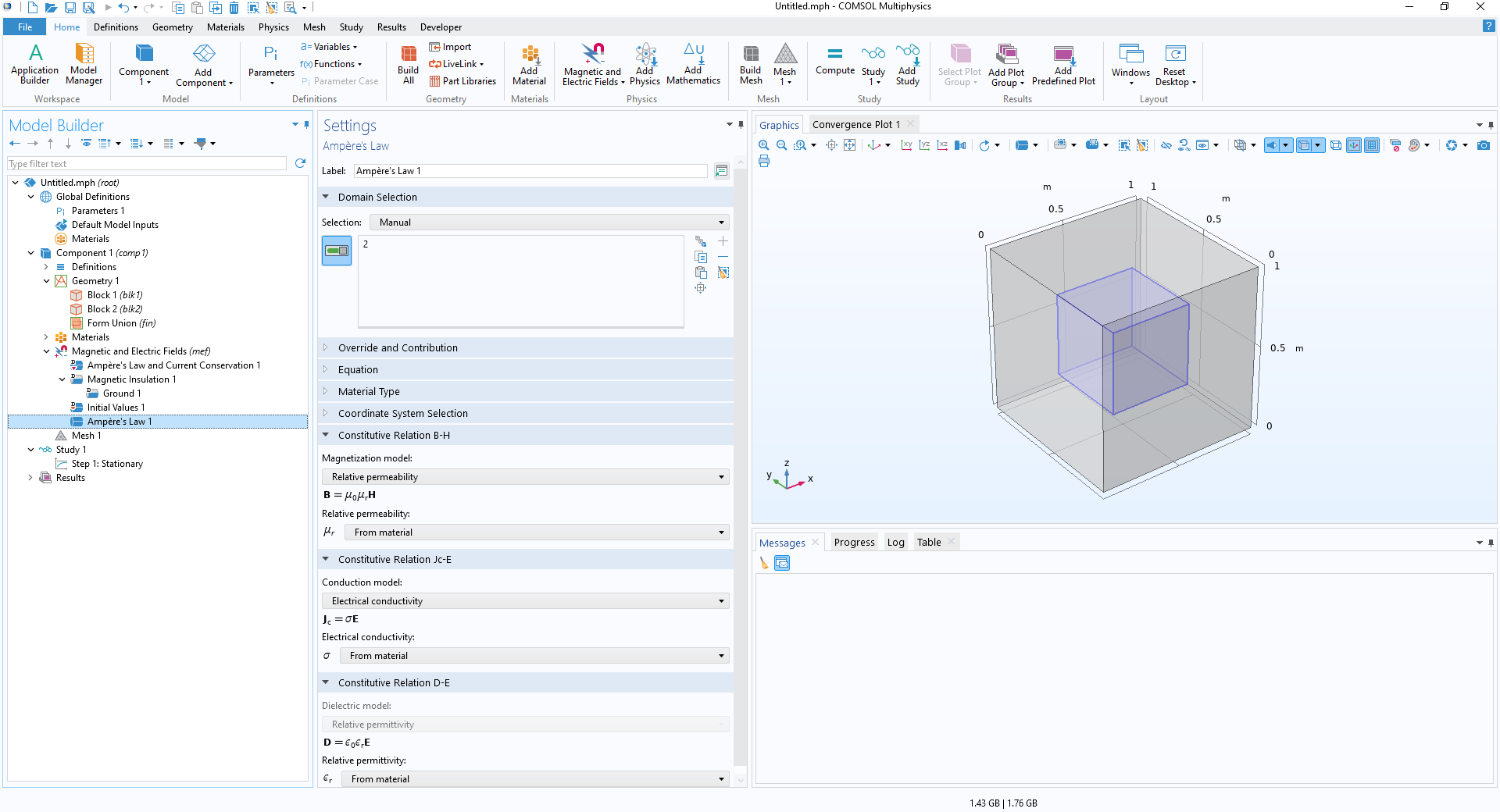
The Magnetic and Electric Fields Interface

When added to an MHD model, theMagnetic and Electric Fieldsinterface uses anAmpère's Law and Current Conservationnode to define the equations that are being solved for. The default external boundary condition is that the boundary is magnetically insulated and grounded.

A Magnetic and Electric Fields node and Free Space, Magnetic Insulation, Ground, and Initial Values subnodes.
TheMagnetic and Electric Fieldsnode and default subnodes.

As bothandare solved for, all boundary conditions have to define how they relate to both of these variables. Additionally, only certain combinations of constraints are physically realistic. For this reason, all constraints onare applied as attributes to a constraint on. This is seen in the default external boundary conditions where theGroundfeature is an attribute to theMagnetic Insulationfeature. For more information, including a list of all the available combinations of magnetic and electric boundary conditions and what they represent physically, see pages 380–383 of theAC/DC Module User's Guide.

Defining Free Space, Insulators, and Conductors

TheMagnetic and Electric Fieldsinterface includes three formulations of the equations for Ampère's law and current conservation in the model:

Free Space, which is designed to handle calculation of magnetic and electric fields in air.
Ampère's Law, which is designed to handle calculations of magnetic and electric fields in materials with no conduction currents. This one feature can be configured to handle either solid or fluid materials by adjusting theMaterial Typenode. Solid materials should have theSolidmaterial type, and fluid materials should have theNonsolidmaterial type.
Ampère's Law and Current Conservation in FluidsandAmpère's Law and Current Conservation in Solids, which are designed to handle fields in conducting materials. In these domains, the current conservation equation is defined, allowing an electric potential and conduction current to be defined and solved for.

TheFree Spacefeature is normally the default feature defining the equation that is solved in all domains, withAmpère's LawandAmpère's Law and Current Conservationnodes added to override it in insulating and conducting domains, respectively. However, by selecting theMagnetohydrodynamicsinterface, an initialAmpère's Law and Current Conservation in Fluidsfeature is added and applied to all domains, as theMagnetohydrodynamicscoupling is only valid in domains selected in this feature.

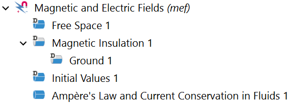
The first step in setting up theMagnetic and Electric Fieldsinterface is ensuring that the correct equation formulations are used in each domain. TheAmpère's Law and Current Conservation in Solidsfeature should be applied to solid conductors; theAmpère's Lawfeature, with the correct material type, should be applied to non-air insulators; and theFree Spacefeature should be applied to any air domain.

The Ampère's Law feature is applied to a domain, which is visualized as a blue cube in the Graphics window. Applying theAmpère's Law feature to a domain in the model to prevent conduction currents flowing in it.

Discretization

TheDiscretizationoption in the settings for theMagnetic and Electric Fieldsinterface defines the order of the function used to discretize the continuous physics into a discrete problem. The discretization for bothandcan be set independently. The default discretization for bothandis quadratic, but for highly nonlinear problems, such as MHD models, it can be useful to decrease the order to linear. If theMagnetic and Electric Fieldsinterface was created by adding theMagnetohydrodynamicsinterface to the model, the discretization will have been reduced to linear.

The Magnetic and Electric Fields Settings window showing the magnetic vector and electric potential set to linear. TheDiscretization setting in theMagnetic and Electric Fields interface, showing the discretization for theMagnetic Vector Potential andElectric Potential options set toLinear.

When a higher degree of accuracy is needed in the model, it is possible to increase the discretization of one or both of the dependent variables. The model will take longer to solve on the same mesh as it would at a lower discretization, but there will also be reduced error.

Defining Uniform Background Fields

In theMagnetic and Electric Fieldsinterface, a background field is defined using theBackground Magnetic Flux Densityfeature. Adding this feature defines the magnetic flux density in the entire model to be equal to, whereis a specified uniform flux density. In addition, on the boundaries where theBackground Magnetic Flux Densityfeature is added,is constrained to have no component normal to the wall so that the component ofnormal to the wall is equal to the component ofnormal to the wall. That is,on the boundaries.

This is very similar to defining the relative field formulation in theMagnetic Fieldsinterface along with theExternal Magnetic Potentialfeature on the boundaries. However, in this case, it is still the total field, which is solved for rather than the relative field.

Additional Information Note: TheBackground Magnetic Flux Densityfeature is a boundary condition, however it effects the fields in the domains of the model.

The mathematical constraint used in the feature is that for the magnetic vector potentials corresponding toand,. The boundary condition only guarantees that the tangential components ofandare equal. Their normal components might deviate depending on specific situations.

While the normal components are only equal on the boundaries, the feature has the effect of generating a uniform background flux density across the entire modeling domain by using the principle of superposing fields. This is because a flux density, which can be written as, satisfies both the equations and the boundary condition thatas long ason these boundaries. This functions very similarly to the reduced field formulation in theMagnetic Fieldsinterface; however, it is still the total field that is solved for in this case.

The Background Magnetic Flux Density Settings window showing the boundaries selected and the Graphics window showing the boundaries highlighted in blue. Applying theBackground Magnetic Flux Density boundary condition.

TheBackground Magnetic Flux Densityfeature includes the option to define a constraint onto give a boundary condition on the electric field. The default isGround, which can be interpreted as the model being enclosed in a perfectly conducting box.

The context menu is opened from the Background Magnetic Flux Density node to show the options that can be used in combination. Available constraints on V that can be used in combination with theBackground Magnetic Flux Density condition.

Choosing the appropriate condition ondepends on the physical context of the model:

If the boundary is the inlet or outlet, and the flow is normal to the boundary, then the EMF current flow must be tangential to the boundary. TheElectric Insulationcondition is then appropriate.
If the boundary is a physical electrode, one of theGround,Electric Potential,Floating Potential, orTerminalfeatures should be used as appropriate.
If it is the boundary between conducting wall domains that is physically modeled, and a nonmodeled infinite air domain is assumed to be perfectly insulating, theElectric Insulationfeature should be used.
In the case of pipe or duct flow models, where only the fluid is modeled and the walls are a mixture of perfectly insulating and perfectly conducting materials that will be handled through boundary conditions, the choice is dependent on the wall conductivity and placement.

Defining Wall Behavior When Only Fluid is Modeled

In the case where only the fluid domain is modeled, the wall conductivity is defined by which constraint onis added to theBackground Magnetic Flux Densitynode. The following features can be used:Electric Insulation,Ground, orFloating Potential. Which of these features is required can be identified by considering the conductivity of the physical wall material:

If a wall is electrically insulating, then theElectric Insulationcondition is required.
If all of the walls are conducting, then theGroundcondition is required for all of them.
If some of the walls are conducting, then theGroundcondition is required for one wall, while either theFloating PotentialorGroundcondition is required for the other conducting walls depending on whether the solution to the physics requires them to be at 0 V relative to the first wall that was grounded or at a nonzero potential relative to it.

In cases where only some of the walls are conducting, it can be very difficult to assess which walls need to be grounded and which need a floating potential — a fixed, nonzero potential that the model will solve for — assigned to them. The easiest method for evaluating this is to solve a version of the model that uses a finite but very high conductivity for the wall material and plot the potential across the cross section of the duct. Ifon the fluid boundary in this version of the model evaluates to zero, then it should be grounded in the version using the perfect conductors; otherwise, it should have aFloating Potentialcondition assigned to it. OneFloating Potentialshould be used for each set of connected conducting boundaries.

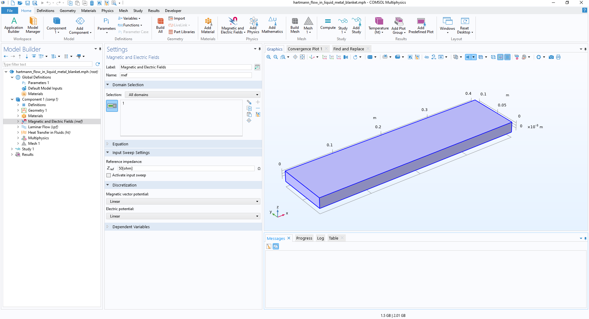
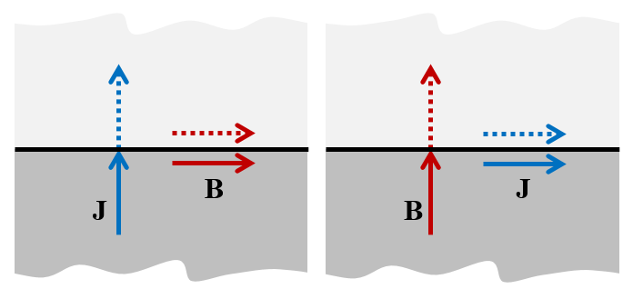
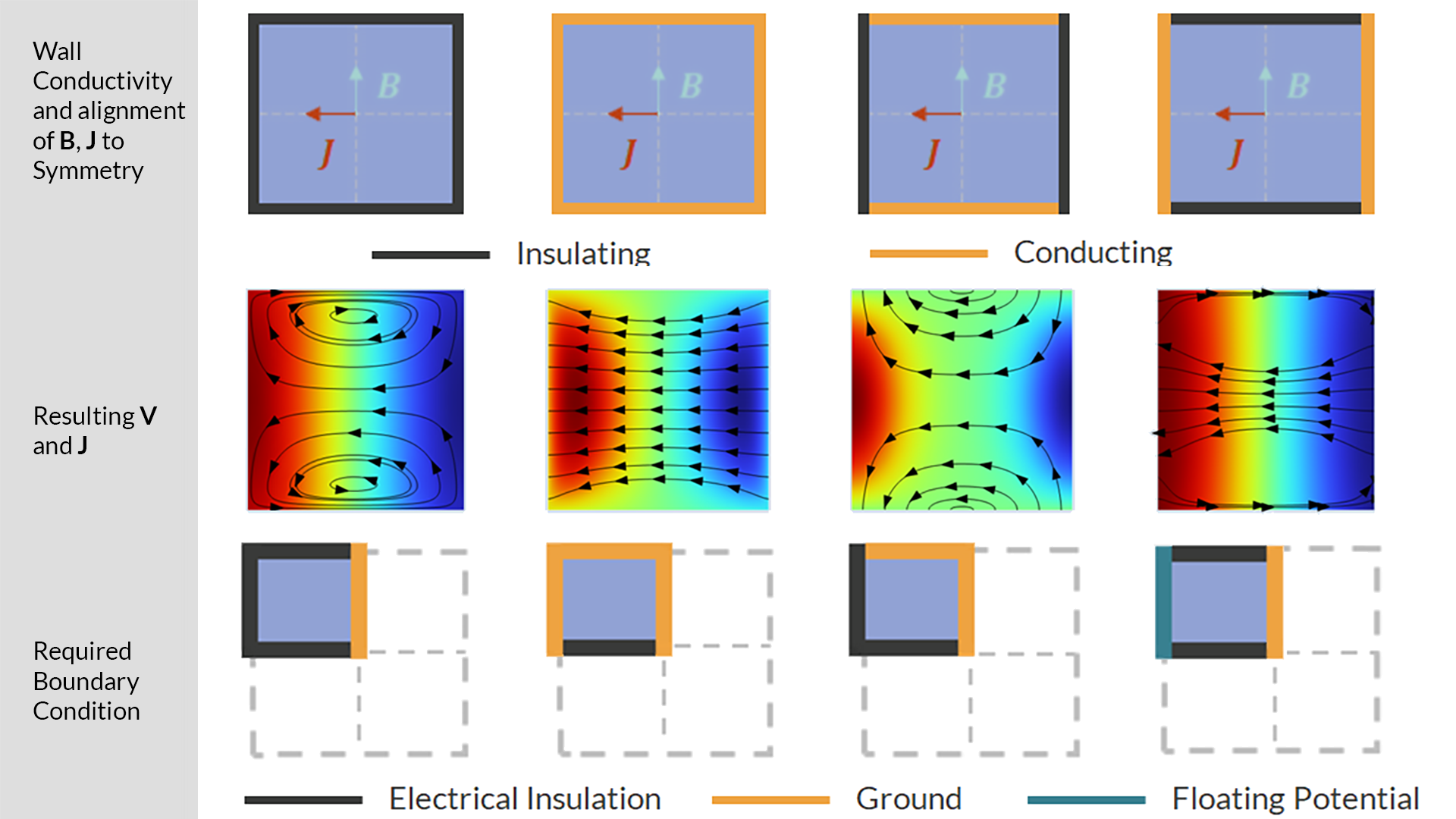
For flow in a rectangular duct with a vertical background magnetic field, there are four common combinations of wall conductivity: all conducting; all insulating; conducting side walls with insulating Hartmann walls; and insulating side walls with conducting Hartmann walls. Assuming thatis aligned with the z-axis, the Hartmann walls are the top and bottom walls of the duct, and the side walls are the vertical walls. The combinations ofGround,Electric Insulation, andFloating Potentialconditions that are required for each of these arrangements of walls are shown below, along with the distribution ofthey generate on the cross section.

A grid of varying wall conductivity combinations and the boundary conditions required for each.
Identifying the boundary conditions for different wall conductivity combinations for square duct flow by considering the value ofon each of the boundaries.

Using Symmetry

Capitalizing on symmetries in a system to reduce the modeling domain can significantly reduce computation time and memory costs by decreasing the size of the geometry and the resulting number of degrees of freedom. Many interfaces includeSymmetryboundary conditions; however, because theMagnetic and Electric Fieldsinterface constrains both the magnetic and electric fields on the symmetry plane, it does not include aSymmetryboundary condition. Instead, you need to identify how the symmetry is reflected in the magnetic and electric fields and choose a combination of boundary conditions that will give the desired field shape.

There are two forms of symmetry for electromagnetic fields. For a symmetry plane with normal, these are:

Symmetry,, so that the current is normal to the symmetry plane and the magnetic field is tangential to it
Antisymmetry,, so that the magnetic field is normal to the symmetry plane and the current is tangential to it

Two images showing the relationship of J and B with solid and dotted colored arrows.
The relationship ofandto the symmetry plane for the case of symmetry (left) and antisymmetry (right).

Boundary conditions can be used to constrainandto be tangential or normal to the boundary as is appropriate for whether it is a symmetry or antisymmetry condition:

Symmetry:Magnetic Insulationcondition to constrainto be tangential, with aGroundattribute that constrainsto be normal
Antisymmetry:Perfect Magnetic Conductorcondition to both constrainto be normal andto be tangential

In the case where there is a uniform background magnetic field, the background field must already obey the symmetry or antisymmetry condition, and so it is possible to use theBackground Magnetic Flux Densitynode with an appropriate constraint on V to define the symmetry plane:

Symmetry:Background Magnetic Flux DensityandGround
Antisymmetry:Background Magnetic Flux DensityandElectric Insulation

The easiest method of identifying whether a symmetry plane is a symmetry or antisymmetry plane is to plotandin the system and identify whether they are normal or tangential to the plane. If the perfect insulator and perfect conductor wall conditions described here are being used, it is also necessary to plotand identify if the conducting walls will have theGroundorFloating Potentialfeature applied to them.

A grid of wall conductivities and alignments to B and J with the boundary conditions required for each case.
Identifying the boundary conditions required to use the two planes of symmetry in a square duct flow model by considering the value ofand whether the symmetry plane is a symmetry or antisymmetry plane.

Combining Uniform Background Fluxes and Periodic Systems

When modeling the flow of liquid metals in long ducts, it is advantageous to utilize the periodicity of the system to model only a small section of the larger system. ThePeriodic Conditionfeature allows periodic structures to be modeled by enforcing that the magnetic vector potentialand the scalar potentialmatch on the source and destination boundaries. It can also be used in combination with theBackground Magnetic Flux Densityfeature to model periodic systems within uniform background fields. However, you need to note how the two features interact and make some changes to the default settings to ensure they contribute together correctly.

The first boundary condition that should be applied to the system is thePeriodic Condition, which is applied to the faces on either side of the periodic cell. These faces must be parallel, and the displacement vector between them defines the axis of periodicity. The modeling is simplest if this axis is aligned with thex-,y-, orz-axis.

The Periodic Condition Settings window with the selected boundaries shown in blue in the Graphics window. Applying thePeriodic Condition to a duct flow model. The periodicity and the motion of the fluid is along thex -axis.

TheBackground Magnetic Flux Densitycondition is then applied to the external boundaries that are not the periodic faces. The necessary constraints on V can be applied with it.

The Background Magnetic Flux Density Settings window with a background field configured in the z direction on the nonperiodic faces shown in blue in the Graphics window. Adding the uniform background field in thez direction to the duct flow model by defining aBackground Magnetic Flux Density feature on the nonperiodic faces.

TheBackground Magnetic Flux Densitynode applies the field by identifying a magnetic vector potentialthat corresponds to the specified background flux density,. The boundary condition then applies this as a constraint on the solved for vector potentialby specifying that, whereis the surface normal. For any, there are infinitely many possible, and it is thus necessary to make a choice of which one to use.

The default choice used by the equations is to use

This is generally a good choice, as it does not introduce a preferred direction into the equations, splitting the contribution toevenly betweenand, and similarly forand. However, it interacts poorly with the periodic condition, where specific directions in the model have to be considered.

If it is assumed that the periodic axis lies along thex-axis, and the periodic cell runs over the range, then evaluatingon either side of the periodic cell gives

It is seen that any term inthat involves the coordinate parallel to the periodicity axis will not meet the periodicity requirement. This has the effect of inducing an additional contribution tothat will cancel out these terms to maintain the periodicity. The effective background field that is then applied is effectively

when the periodicity axis is thex-axis, with similar expressions for if the periodicity axis follows they- orz-axis.

This effective potential has the effect that while a background field aligned with the periodicity axis is applied at full strength, any field normal to it only contributes at half of its full strength. To resolve this issue, it is possible to adjust the vector potential used by theBackground Magnetic Flux Densityto a potential that defines the flux densitywhile also meeting the periodicity requirement. When the periodic axis is along thex-axis, the vector potential should be set to:

Similar definitions can be made for when the periodic axis aligns with they- orz-axis.

To set this as the vector potential used by theBackground Magnetic Flux Densityfeature, it is necessary to enableEquation Viewto have access to the equations used by the feature and edit them. This is accessed by enabling theShow Equation Viewsetting in theShow More Optionsmenu accessed from the top of the model tree. AnEquation Viewnode is then generated under theBackground Magnetic Flux Densitynode. Opening the settings for thisEquation Viewnode, the equations defining the background vector potential are then available. The expressions can then be edited to be defined as the corrected potential.

The Equation View Settings window under the Background Magnetic Flux Density node. Editing the expressions for the background vector potential to the corrected form for a system that is periodic along thex -axis.

Constraining Models for Convergence

Since the electric and magnetic fields are defined as the gradient and curl ofand, respectively, it is possible to add an appropriate term to each and still have the same electric and magnetic field before boundary conditions are considered. This means that in many cases, the solution to the problem is not unique. This can cause issues with the solver not converging.

To resolve this issue, it is necessary to ensure the choices ofandare constrained in some way.

To constrain, it is necessary to fix the electric potential in the model in some way. If there is already aGround,Electric Potential, orTerminalboundary condition in the model to connect the model to an electrode at a known potential, then this will also provide the constraint on, ensuring the unique solution for the solver.

Ifis not constrained to a known value on a boundary, it is necessary to constrain it at a point in the model, using theGroundpoint feature. This will constrainby acting as a reference point for measuring the potential in other parts of the model, without it acting as a source or sink of current.

Ifis not constrained, it is still possible to solve theMagnetic and Electric Fieldsinterface, but an iterative solver is required. If it is desired to use aDirectsolver, it is necessary to constrainby applying gauge fixing via aGauge Fixing for A-Fieldnode. This introduces an additional variable that is used to fix the model in the Coulomb gauge.

For more information on gauge fixing, see the following blog posts: "What Is Gauge Fixing? A Theoretical Introduction" and "How Do I Use Gauge Fixing in COMSOL Multiphysics^®?".