学习中心

Performing an Uncertainty Propagation UQ Study

---

In this part of our uncertainty quantification (UQ) course, we will continue our analysis of the steel bracket model from Parts 2–3, now focusing on an uncertainty propagation analysis of the two most influential input parameters.

The sensitivity analysis discussed inPart 3identified the misalignment angle as being sensitive to variations in the side length (ls) and cross-plate width (wp). We will now conduct a more detailed analysis of how the misalignment angle responds to changes in these parameters. Specifically, we would like to understand how the probability distributions of the side length and cross-plate width impact the probability distribution of the misalignment angle. This analysis will ultimately enable us to assess the risk of an excessive misalignment angle.

Uncertainty Propagation

Similar to the transition from a screening analysis to a sensitivity analysis, there is no need to reenter all of the uncertainty quantification parameters when moving from a sensitivity analysis to uncertainty propagation. Instead, you can define a newUncertainty Quantificationstudy for uncertainty propagation by reusing the information from the sensitivity study. The outcome of the uncertainty propagation analysis will include statistical properties related to the variation of the misalignment angle, such as the mean and standard deviation. Additionally, the probability density function of the misalignment angle will be visualized using a kernel density estimation (KDE) plot.

Open the Model and Add the Study

To begin the uncertainty propagation analysis, start by opening the model file for the UQ structural and sensitivity analysis of a bracket fromPart 3. Save the file and rename it tobracket_uq_static_structural_and_uncertainty_propagation.mph.

Right-clickStudy 3>Uncertainty Quantificationand selectAdd New Uncertainty Quantification Study For Uncertainty Propagation, as shown in the figure below. This step generates theStudy 4node, where the uncertainty propagation analysis settings are available.

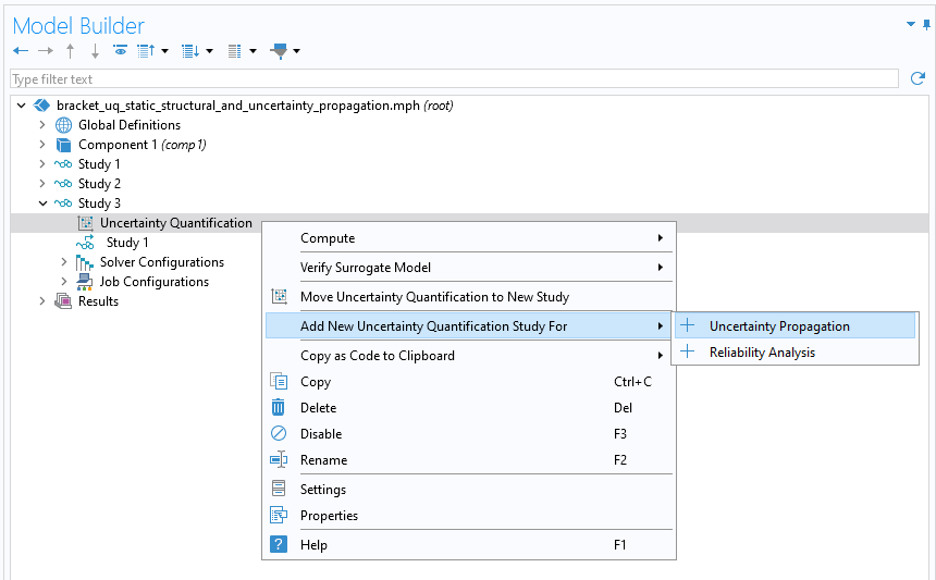A screenshot of part of the model tree with the menu options for the Uncertainty Quantification study node expanded and the Uncertainty Propagation option selected.

Adding the UQ study type for uncertainty propagation.

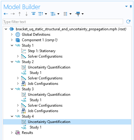
Study 4is the thirdUncertainty Quantificationstudy. This study has theUncertainty propagationoption enabled.

In theSettingswindow for theUncertainty Quantificationstudy, the UQ study type is automatically set toUncertainty propagation. The settings for theQuantities of InterestandInput Parameterssections will automatically be copied over from the sensitivity analysis ofStudy 3. However, for the uncertainty propagation analysis, we will keep only the side length and cross-plate width as input parameters. To remove the other parameters, select each one individually and click theDeletebutton located beneath the table in theInput Parameterssection. After this step, the list of input parameters should match the figure shown below.

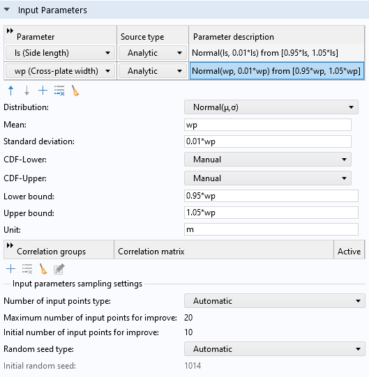
The two input parameters used for the uncertainty propagation analysis.

To accelerate the uncertainty propagation analysis, this UQ study type also uses a surrogate model, specifically an adaptiveGaussian Process(GP) surrogate model. A GP surrogate model approximates the relationships between inputs and outputs with a statistical model that can quickly predict the output for any given set of input parameters, even for values that the finite element model hasn't directly solved for. This approach significantly reduces computational cost while maintaining accuracy, as the GP surrogate model adapts to the underlying data, capturing the most important characteristics of the model's behavior under uncertainty.

During the uncertainty propagation study, the creation of the GP surrogate model is automated, ensuring that only a minimal number of model evaluations are required. After computation, the surrogate model becomes available underGlobal Definitions. In this case, the surrogate model defines a single GP function that can potentially be reused for other purposes through a function call. The default selection for theCompute actionsetting isImprove and analyze. TheImprove and analyzesetting automatically reuses previously computed uncertainty quantification results as a way to speed up the computation. However, here we will change this selection toCompute and analyze(shown below) since we already modified the input parameters from the sensitivity analysis study, and since the existing data used to train thePolynomial Chaos Expansionmodel is not consistent with our current settings.

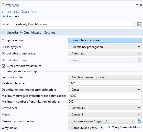
The uncertainty propagation settings in theUncertainty QuantificationstudySettingswindow. Here, the selection for theCompute actionsetting has been changed toCompute and analyze.

During the computation, the input parameter space is sampled using a Latin-hypercube-sampling-based design of experiments method. The GP surrogate model is adaptively improved during this process until either the tolerance or the maximum number of sample points is reached. You can read more about the GP surrogate model type in the surrogate modeling course part oncreating a multiphysics-driven Gaussian process surrogate modeland the surrogate modeling theory course part onGaussian process surrogate models.

Run the Simulation and Analyze the Results

To begin the uncertainty propagation computation, right-clickStudy 4and selectCompute. The computation takes about 10 minutes depending on the hardware. The default plot is a KDE plot (shown in the figure below), which represents the estimate of the probability density function for the misalignment angle. You can think of the KDE as a smooth form of a histogram showing an estimate of the probability density function of the quantity of interest, given the input parameters and their distributions. We can see that the most likely misalignment angle is around 0.09.

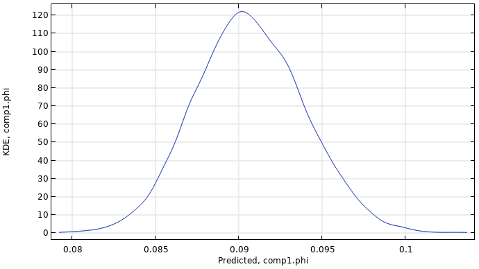
A KDE plot of the misalignment angle.

Statistical values for the uncertainty propagation analysis are available in theQoI Confidence Intervaltable, as shown in the figures below. The table gives a value of 0.003 degrees for the standard deviation, indicating a quite small variation around the mean value of 0.09 degrees.

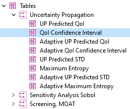
The location of theQoI Confidence Intervaltable under theResultsnode.

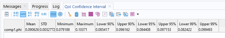
The mean, standard deviation, minimum, maximum, and confidence interval values computed from the uncertainty propagation analysis.

Note that the results are somewhat different for the model version without fillets: The mean and standard deviation values are slightly higher for the version without fillets.

In the next part, we will further refine the analysis by using the reliability analysis option. This will enable us to, for example, estimate the probability that a quantity of interest exceeds a certain threshold.

UQ Study Warnings and Errors

When the computation is complete and the maximum number of iterations or input points has been reached without meeting the relative tolerance value, a warning is displayed in theLogwindow, and a warning triangle appears next to the model tree node underJob Configuration>Uncertainty Quantification, as shown in the figure below.

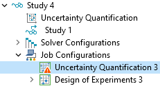
The warning indicator shows that the relative tolerance criterion was not met.

In most cases, the most effective way to improve the accuracy of a surrogate model is by increasing the number of input points, regardless of the type of UQ study. However, this requires additional finite element model evaluations, leading to longer computation times. The default tolerance is set very low, and achieving this level of accuracy for the surrogate model may not be necessary or feasible. Instead, one should balance computation time and accuracy by increasing the number of input points as much as possible without exceeding a reasonable computation time.

For a UQ study that uses a GP surrogate model, not having reached the relative tolerance is just one of several reasons for a warning or error message to be displayed. The warnings and error messages are listed inJob Configurations>Uncertainty Quantification>Settingswindow >Error, as shown in the figure below. Note that these warning messages may not indicate that there is anything wrong with the model but are merely alerts triggered when various conditions or thresholds are met.

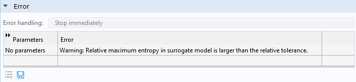
TheErrorsection of theSettingswindow for theJob Configurations>Uncertainty Quantificationnode.

The most common reasons you'll get an error message include:

• A maximum number of surrogate model evaluations was reached before the relative tolerance was met (GP surrogate model only).
• A maximum number of optimization iterations was reached before the tolerance was met (GP surrogate model only).
• A maximum number of input points (sample points) was reached before the tolerance was met.
• The geometry failed to build, e.g., because a negative radius was requested.
• The mesh failed to build, e.g., because an excessively thin domain was created.
• The solver failed to find a solution, e.g., because the parameters defined an unphysical model.

In theAdvanced Settingssection of theSettingswindow forStudy 4>Uncertainty Quantification, you can request that the UQ study skips parameters that generate an error. To do so, change theError handlingsetting fromStop immediatelytoSkip problematic parameters, as shown in the figure below. This setting enables skipping problematic parameters but will still log all possible errors in theErrorssection.

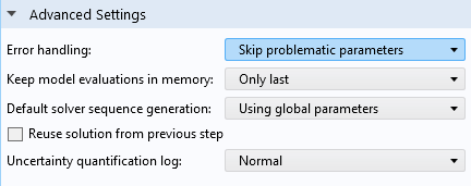
The error handling settings in theSettingswindow for theUncertainty Quantificationnode.

In this part of the course, we have focused on performing an uncertainty propagation UQ study. The next part of the course will focus on performing a reliability analysis.