学习中心

Creating a Polynomial Chaos Expansion Surrogate Model from Imported Data

---

To continue the process of learning how to create surrogate models in COMSOL^®using imported data, we will now walk through fitting imported data to aPolynomial Chaos Expansion(PCE) surrogate mode. We will use the same dataset that we used in Part 5. This dataset takes the form of a functional surface, and the variables can represent any quantity. The workflow presented here is applicable when the data originates from experimental results.

Note: The Uncertainty Quantification Module is required for this example.

Polynomial Chaos Expansion Overview and Comparison to Gaussian Process Model

PCE surrogate models are widely used for uncertainty quantification (UQ), particularly in sensitivity analyses. They serve as a valuable alternative toGaussian Process(GP) surrogate models, as they do not require hyperparameter optimization or the selection of a covariance function. Instead, PCE involves selecting a predefined probability distribution for each input parameter. Based on these distributions, the method automatically determines an appropriate polynomial basis and expands the quantities of interest within that basis, known as apolynomial chaos expansion. This approach is particularly efficient for sensitivity analyses, as implemented in the Uncertainty Quantification Module, for identifying the most influential quantities of interest. Subsequently, a GP model can be used for more detailed analyses, such as uncertainty propagation or localized standard deviation estimates, focusing on the most influential parameters identified.

Here, we will learn how to create a PCE model. Unlike GP models, a PCE model does not provide pointwise uncertainty. However, using the Uncertainty Quantification Module, we can compute statistical metrics such as the global mean and variance of the surrogate model. For an example of a sensitivity analysis based on a PCE model, see the next part of this course: "Sensitivity Analysis Using a Polynomial Chaos Expansion Surrogate Model".

Fitting Imported Data with a PCE Surrogate Model

Start by loading the GP surrogate model with UQ (gp_experimental_fit_uq.mph) from Part 5. We will continue working on this model, which has the training data stored in theTable 1node.

The training data for this example is stored inTable 1.

First, rename the model topce_experimental_fit_uq.mphand save.

If you have access to the Uncertainty Quantification Module, you can now add aPolynomial Chaos Expansionsurrogate model function. To do this, right-clickGlobal Definitionsand selectPolynomial Chaos Expansionfrom theFunctionsmenu.

Adding aPolynomial Chaos Expansionsurrogate model.

In thePolynomial Chaos ExpansionfunctionSettingswindow, chooseResult tableas theData sourceand then selectTable 1for theResult tablesetting. TheData Column Settingssection will automatically be filled out with defaultArgumentandFunction values:x1,x2, andpce1.

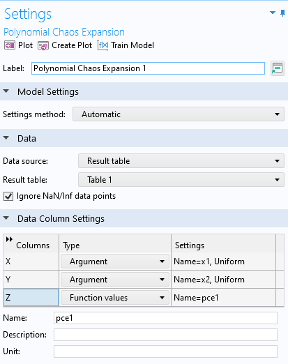
The settings for thePolynomial Chaos Expansionsurrogate model function.

In this case, we will assume that the two input parameters have a uniform distribution in. Click the first row in theData Column Settingstable and type0and10for theLower boundandUpper bound, respectively. Repeat this process for the second row.

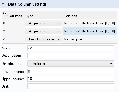
The uniform distribution settings for the input parameters.

At the top of thePolynomial Chaos ExpansionfunctionSettingswindow, clickTrain Model. In this case, this action prompts a warning message that 116 of the 900 training points are excluded. The reason for this is that 116 of the training points are on the boundary of the rectangle. The Legendre polynomial approximation algorithm cannot handle this; it is required that we extend the domain slightly.

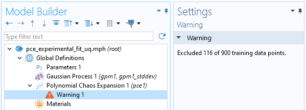
The PCE method gives a warning for data lying exactly on the boundary.

We can extend the domain slightly by introducing a parameter with a small value. Under theParameters 1node, enter a new parameter with the namesmalland the expression1e-6.

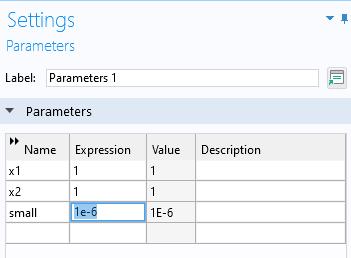
The global parameter for extending the surrogate model region.

Now modify the bounds of the uniform distribution by changing theLower boundandUpper boundvalues to0-small(or just-small) and10+small, respectively, for both input parameters.

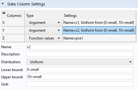
The extended bounds for the uniform distribution.

To generate the surrogate model, clickTrain Modelat the top of thePolynomial Chaos ExpansionfunctionSettingswindow. The computation takes a few seconds. Once it is complete, plot the function by clicking theCreate Plotbutton. The plot can be seen in the figure below.

The Model Builder with the Function 1 plot node selected and the corresponding Settings window and plot visualization displayed.

A visualization of thePolynomial Chaos Expansionsurrogate model created from experimental data.

The dataset appears to vary wildly. However, this is due to the automatic z-axis scaling, and upon further inspection, the function values are within a narrow range between about 1.15 and 1.24.

We are now interested in computing the global mean value and standard deviation. To do this, we need to run theUncertainty Quantificationstudy. The study currently uses the previously computed GP model, which we will now change to the PCE model.

Computing Uncertainty with the Uncertainty Quantification Study

In theUncertainty QuantificationstudySettingswindow, change theSurrogate modelsetting toSparse polynomial chaos expansion. Then, change the PCE function to the one we just trained:Polynomial Chaos Expansion (pce1). Finally, change the option for theCompute actionsetting toAnalyze only. This option enables us to compute statistical properties without retraining the surrogate model.

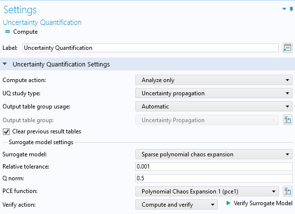
TheUncertainty QuantificationstudySettingswindow, showing the settings for the PCE function.

The default surrogate model forSensitivityisAdaptive Sparse polynomial chaos expansion. However, in this case, we will reuse an existing surrogate model, so the adaptive method will not be invoked. The adaptive method requires the generation of new data points, which is not possible for imported data since there is no finite element model to compute additional data points. Therefore, when we select theAnalyze onlyoption, the adaptive method is automatically disengaged, and there is no need to change this setting. In this example, both theAdaptive sparse polynomial chaos expansionand theSparse polynomial chaos expansionsettings use a nonadaptive PCE method.

Now we are ready to analyze the surrogate model. At the top of theUncertainty Quantificationwindow, clickCompute. Recall that in the case of anUncertainty Quantificationstudy, the sampled variables are output to aQuantities of Interesttable, rather than aDesign Datatable.

When the computation is finished, aKernel Density Estimation (KDE)plot is shown. Recall that a KDE plot is a smoothed histogram plot and represents the probability density function estimate for the function value considering all input values in the region. In other words, the KDE plot shows the most probable function values when the input parameter space is randomly uniformly sampled within the set parameter boundaries.

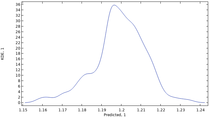
A KDE plot showing the probability density function estimate for the function values of the imported data.

We can also get statistical information from this computation. If not already visible, under theResults>Tablesnode, select theQoI Confidence Intervaltable underUncertainty Propagation.

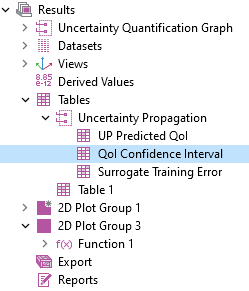
Selecting theQoI Confidence Intervaltable.

TheQoI Confidence Intervaltable contains information about the surrogate model's global mean and standard deviation as well as the minimum, maximum, and various quantile values.

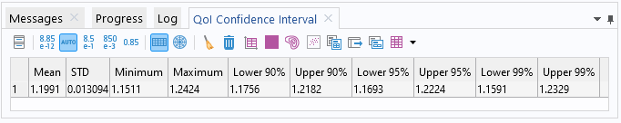
TheQoI Confidence Intervaltable.

The global mean value is computed to about 1.2 and the standard deviation is about 0.013, indicating a near constant dataset. The minimum and maximum values are about 1.15 and 1.24, respectively. Note that these values do not correspond to the original dataset but to the fitted surrogate model function. Furthermore, notice that the computed statistical values are consistent with that of the GP model in Part 5, despite this PCE model being at a coarser level of approximation.