学习中心

Sensitivity Analysis Using a Polynomial Chaos Expansion Surrogate Model

---

In this part of the course, you will learn how to perform a sensitivity analysis of an analytical function, the Ishigami function, using aPolynomial Chaos Expansion(PCE) surrogate model in COMSOL^®. The Ishigami function is a random function of three variables and a well-known benchmark used to test global sensitivity analysis and uncertainty quantification algorithms. The mean, standard deviation, maximum, and minimum values as well as Sobol indices of the Ishigami function can be calculated analytically for the input distributions used here.

The Sobol indices are used in global sensitivity analyses to quantify the contribution of each input parameter to the overall variance of the output. These indices can be used to identify which input parameters have the most significant impact on the function's behavior, enabling more informed decision-making and model refinement. For example, Sobol indices can be used to limit the number of input parameters used in a more detailed uncertainty quantification analysis.

The Ishigami Function

The Ishigami function is:

where,, and where,, andare independent, uniformly distributed random variables in the interval. The function can be visualized in 3D by using, for example, a slice plot as in the figure below.

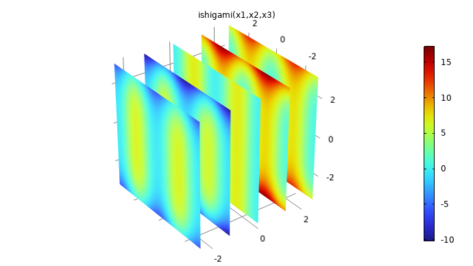
The Ishigami function used for benchmarking.

The mean, variance, maximum, minimum, and a number of other quantities can be computed analytically for the Ishigami function. The MPH-file for the Ishigami function and parameters, available under the reference files for this resource, already has these parameters defined, together with an analytical function definition and the slice plot of the function.

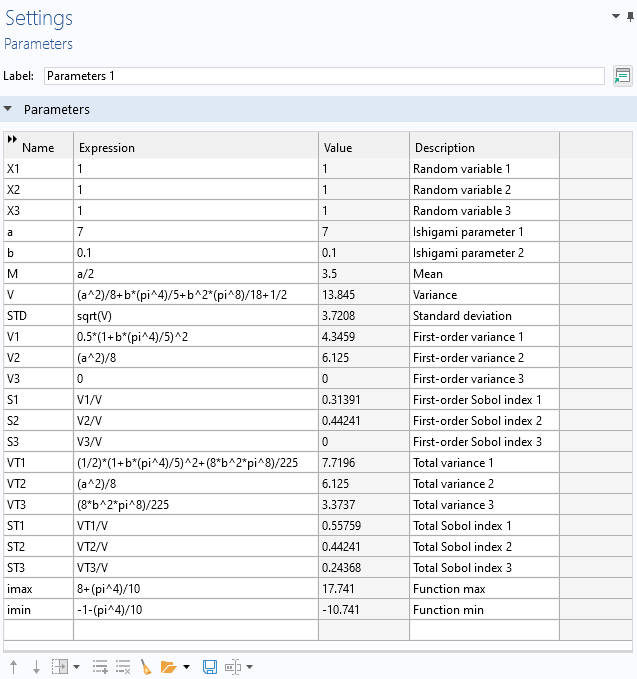
Analytically derived statistical values for the Ishigami function.

Sensitivity Analysis

Let's now start from the model file and perform a global sensitivity analysis of the Ishigami function.

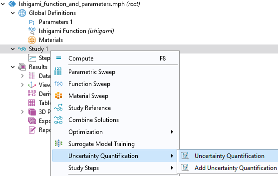
Open the model file for the Ishigami function and parameters. Then, right-click the root node and selectAdd Study.

Adding a study for the Ishigami function.

In theAdd Studywindow, select and add aStationarystudy. Next, right-click theStudy 1node and underUncertainty QuantificationselectUncertainty Quantification.

Selecting theUncertainty Quantificationstudy.

In theUncertainty QuantificationstudySettingswindow, change theUQ study typesetting toSensitivity analysis. There are two sensitivity analysis methods available,SobolandCorrelation. The default option isSobol, which will be the one we use here. In theSurrogate model settingssection, we will use the defaultSurrogate modeloption, which isAdaptive sparse polynomial chaos expansion. ThePCE functionis set toNew, which means that the study will automatically build a PCE surrogate model.

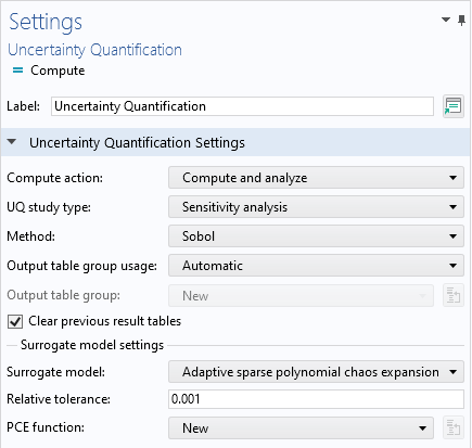
TheUncertainty Quantificationstudy settings for the Ishigami function example.

Next, we will define the quantity of interest, which will be a call to the Ishigami function. In the list of global parameters, the three input parameters,X1,X2, andX3, are already defined. In theQuantities of Interesttable, add a new row, and for the expression enterishigami(X1,X2,X3). In theInput Parameterssection, add the three input parameters withDistributionset toUniformand theLower boundandUpper boundset to-piandpi, respectively, for each parameter, as shown below.

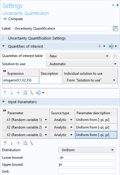
The settings for theQuantities of InterestandInput Parameterssections.

We are now ready to perform the analysis. To do so, right-clickStudy 1and selectCompute. The computation takes a few seconds. The default plot is a Sobol index plot, which shows the first-order and total Sobol indices for each parameter in a bar graph, as shown in the figure below. For each parameter, the first-order index is to the left and the total index is to the right.

The Model Builder with the corresponding Settings window and Graphics window, which displays a bar chart with a set of two blue, green, and red bars.

The Sobol index plot for the Ishigami function.

The first-order Sobol index corresponds to the proportion of the total variance in the output that is attributed to a single input parameter, excluding interactions with other parameters. The total Sobol index corresponds to the proportion of the total variance in the output that is attributed to an input parameter, including both its main effects and all its interactions with other parameters. For more in-depth information on Sobol indices, see our resource that details "More on PCE Surrogate Models, Sensitivity Analysis, and Sobol Indices".

The Sobol indices are displayed in theSoboltable under theResultsnode in theSensitivity Analysis Sobolgroup table. The computed values are consistent with the analytical ones stored in theGlobal Definitions>Parameterstable.

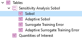
Selecting theSoboltable.

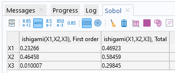
TheSoboltable containing the first-order and total Sobol indices.

For the parameter, we can see that both the first-order and total Sobol indices are relatively significant. The first-order Sobol index indicates a substantial direct contribution ofto the output variance. The total Sobol index suggests thathas a significant impact on the output, both directly and through interactions. The conclusions forare similar.

For the parameter, the relatively small value of the first-order index indicates it does not have any (or nearly any) direct contribution to the output variance. However, the relatively higher value of the total Sobol index implies thatcontributes significantly to the output variance through interactions with other variables. This can also be seen directly from the expression for the Ishigami function:

.

Here,andoccur in their own terms, whereasonly occurs in an interaction term with.

The PCE Surrogate Model

After the computation, a PCE surrogate model is available under theGlobal Definitionsnode.

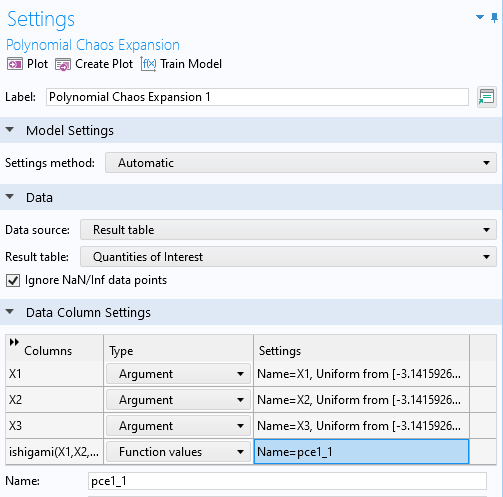
The PCE surrogate modelSettingswindow.

TheInformationsection displays theEstimated errorfor the PCE surrogate model — in this case, the error about 7e-4. The estimated error is based on the so-calledleave-one-out cross-validation error.

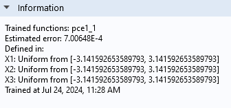
TheInformationsection for the PCE surrogate model.

Plot the surrogate model by clicking theCreate Plotbutton at the top of thePolynomial Chaos ExpansionfunctionSettingswindow. The plot will show some artifacts compared to the original plot, due to the fact that the PCE surrogate model is highly optimized by the adaptive algorithm that only includes the essential polynomial terms in the chaos expansion. For more information, see our resource "More on PCE Surrogate Models".

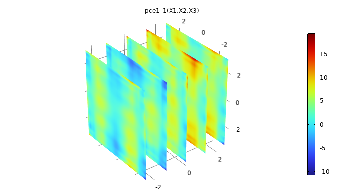
A plot of the PCE surrogate model.

We can increase the accuracy of the model by using a larger number of samples for the input parameters. To do so, in theUncertainty QuantificationstudySettingswindow, in theInput Parameters sampling settingssection, change theNumber of input points typetoManual. Change the values for both theMaximum number of input pointsand theInitial number of input pointsto200. This will force the algorithm to sample the Ishigami function in 200 points. ClickComputeto run the study again.

After the computation, we can compare the surrogate model to the original function by plotting the expressionabs(ishigami(x1,x2,x3)-pce1_1(x1,x2,x3)). This is shown in the figure below.

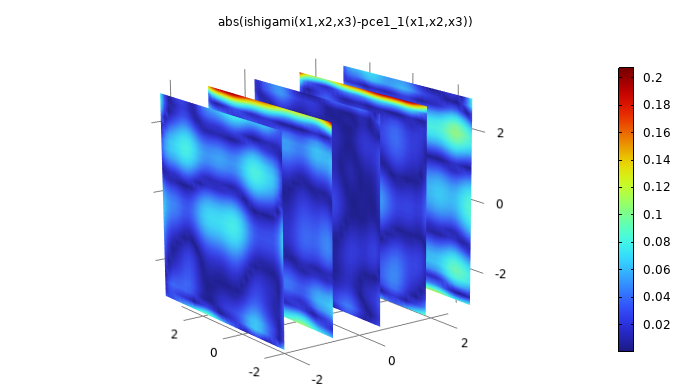
A plot comparing the PCE surrogate model to the Ishigami function.

The maximum pointwise error is about 0.2, which is about 1% of the maximum absolute value of the Ishigami function. To create this plot, right-click3D Plot Group 1and selectDuplicate. In theDataset>Grid 3D 1settings, change theFunctionsetting toAll. This is required so that theGrid 3D 1dataset can recognize the surrogate model function. In the3D Plot Group 4>FunctionplotSettingswindow, change theExpressiontoabs(ishigami(x1,x2,x3)-pce1_1(x1,x2,x3)). Also change theDescriptionsetting to the same expression. Finally, in the3D Plot Group 4nodeSettingswindow, change theTitleto the same expression (alternatively, change theTitle typesetting toAutomatic).

Working with the Ishigami function mimics working with a finite element model in that we can use an adaptive method to iteratively compute more data points. In other words, this example using the Ishigami function is conceptually similar to an uncertainty quantification analysis of a finite element model (or other numerical models). This approach differs from working with imported experimental data. In the case of experimental data, we have to "work with what we have", and the only way to obtain additional data points is to perform additional experiments.