学习中心

Creating Spatially and Time-Varying DNN Surrogate Models

---

Building uponPart 3of this course, where a multiphysics-driven deep neural network (DNN) surrogate model was created, this part will demonstrate how to develop a surrogate model that accurately captures important features of the same thermal actuator model. Using efficient geometry sampling, a DNN surrogate model can be trained to predict voltage, temperature, displacement, and stress fields over a wide range of input parameters. Once trained, the surrogate model can replace the original finite element model, producing near-instantaneous results as input parameters change. We will also briefly discuss time- and frequency-domain sampling.

Note: This demonstration requires functionality in version 6.3 of COMSOL Multiphysics^®.

Generating Space-Dependent Surrogate Model Training Data

In Part 1 of this course, we discussed the fact that we can, in an abstract fashion, view a parametric COMSOL model as a series of functions:

...,

and

whereare the input parameters, which could be length, width, material conductivity, coordinate, etc., andare various output quantities that we are interested in, such as temperature, mechanical stress, or electric potential.

To use a DNN model to reconstruct a field throughout a computational domain, we need to allow some inputs,, to represent spatial coordinates. One approach to generate this data is to treat the spatial coordinates as parameters and let design of experiments (DOE) algorithms sample randomly in space during data generation. However, this approach is inefficient, as each sampled point requires solving the entire model, and only the field values at those specific points are retained, while all other computed field values are discarded.

Let's explore further why this method is inefficient. Suppose we are constructing a surrogate model for a thermal actuator where, just as in Part 3, the actuator lengthand applied voltageare input parameters. Additionally, assume we want the surrogate model to reconstruct the full temperature fieldinside the actuator. In other words, our goal is to build the following surrogate model:

In order to train such a surrogate model, we need to sample a large number of, say,, values. The full finite element model needs to be solvedtimes, once for each parameter combination. This generates the following table:

Sample Number	Outputs	T	Inputs	L	DV	x	y	z
1
2
3
...		...		...	...	...	...	...
...		...		...	...	...	...	...

In this approach, each row is generated by the DOE algorithm combined with a finite element solution. The issue is that to obtain a single temperature value, we must solve the entire finite element model, a step that cannot be bypassed. While the finite element results provide temperature values throughout the actuator volume, a direct DOE method that includes spatial coordinates in the sampling will retain only one temperature value per sampling point,. A more efficient approach would be to allow only the parameters driving the model, such asand, to be set by the DOE sampling and, for each finite element solution, store all the resulting temperature values:

...,

and

whereis the number of finite element mesh vertices (or sampling grid points).

With this revised method, we can represent the data in the following table format:

Sample Number	Outputs	T	Inputs	L	DV	x	y	z
1
2
3
...		...		...	...
...		...		...	...

Each row in this table compactly representsrows of detailed data, corresponding to each mesh vertex. Thus, the full table will containrows of data, whereis the number of finite element model computations. In this revised approach,(the number of sample points) can be much smaller than(from the previous method) while still achieving the same surrogate model accuracy. Generally, a similar sample set can be achieved as before if.

For instance, if the mesh hasvertices and we runsimulations, we would generate a table withrows. A DNN surrogate model can easily handle this amount of data. In contrast, allowing the DOE algorithm to control all input parameters, including coordinates, would require solving the full finite element model 8 million times — an impractical computation.

Efficient Geometry Sampling: Thermal Actuator Surrogate Model App Overview

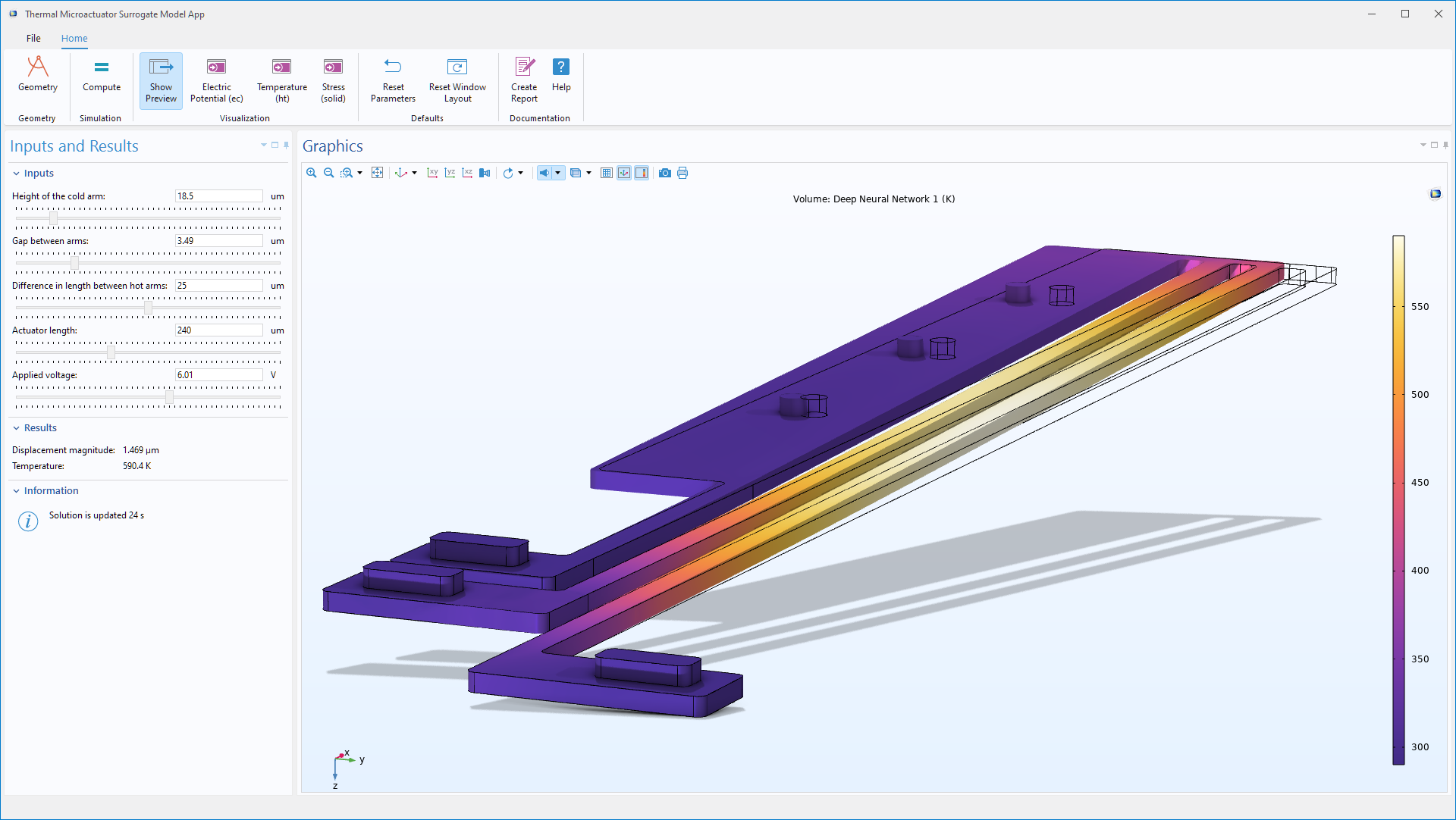
In the Application Libraries, under theCOMSOL Multiphysics> theApplicationssection, theThermal Actuator Surrogate Model appdemonstrates theGeometry Samplingfeature. The figure below shows the app's user interface, where you can adjust four geometric parameters and the applied voltage. A DNN surrogate model retrieves field values near-instantaneously within the entire actuator geometry, with an option to compute the full finite element model for comparison. Note that the parametric CAD geometry and finite element mesh are necessary for displaying the field.

A screenshot of the UI for the thermal microactuator surrogate model simulation app.

The Thermal Actuator Surrogate Model app demonstrating the use of a DNN surrogate model to reconstruct spatially varying field quantities.

The settings for geometry sampling are specified under theDefinitionsnode in theGeometry Samplingfeature, as shown in the figure below. You can choose to sample within one or more domains, boundaries, edges, or points. In this case, only one domain is available, and it is selected for sampling.

A screenshot of the COMSOL Multiphysics UI with the thermal microactuator model opened and the Geometry Sampling feature selected in the model tree.

TheGeometry Samplingfeature used by theSurrogate Model Trainingstudy for efficient data generation.

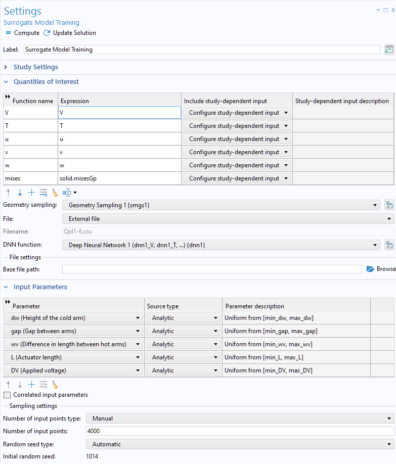
The figure below shows theSurrogate Model TrainingstudySettingswindow, where each quantity of interest references theGeometry Samplingfeature. Selecting a row in theQuantities of Interesttable displays the sampling properties for that specific quantity. Computed data is stored either within the model as an embedded file or externally on the file system. The input parameters are uniformly sampled, and 4000 computations (input points) are specified.

Note that in this app, the embedded model was modified after training the DNN function: theNumber of input pointsvalue in theSurrogate Model Trainingstudy was reduced from 4000 to 1 before recomputing and then disabling the study. This change, made to reduce disk space usage, decreased the embedded CSV file size from 2.6 GB (approximately 8 million rows of data) to less than 500 KB while preserving the trained DNN function.

As a result, the embedded CSV file does not contain the full training data, and the settings in theSurrogate Model Trainingstudy do not fully reflect this modification. To reconstruct the complete dataset, rerun the study with all 4000 input points. For a detailed example and full workflow description, see the documentation for the modeltubular_reactor_surrogate.

The Settings window for the Surrogate Model Training Study.

TheSurrogate Model Trainingstudy settings for the thermal actuator model.

The figure below shows the first rows of the data file generated by theSurrogate Model Trainingstudy.

A screenshot of a text file containing a set of numerical data.

The first few rows of the data file generated by theSurrogate Model Trainingstudy.

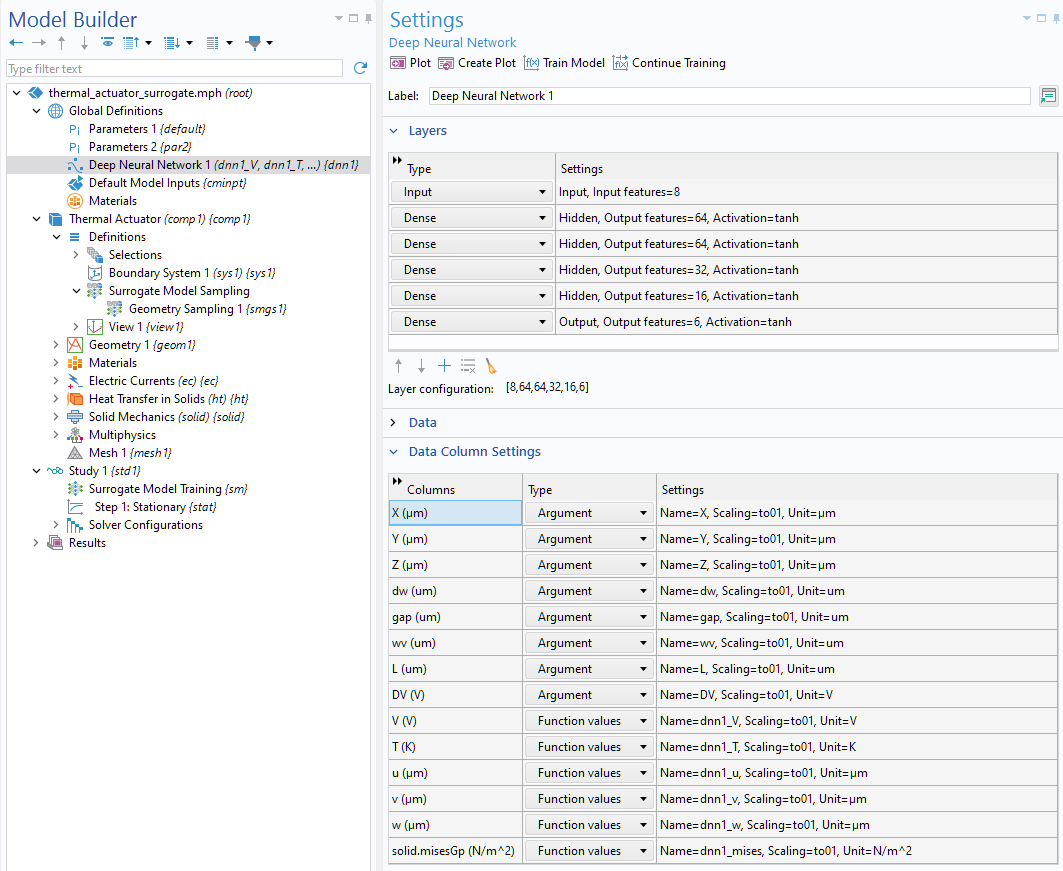
The DNN surrogate model has 8 input features, 6 output features, and 4 hidden layers, which schematically can be represented as. Each layer uses theactivation function, as shown in the figure below. In theData Column Settingssection, theQuantities of InterestandInput Parametersfrom theSurrogate Model Trainingstudy are displayed. The first three columns, originating from theGeometry Samplingfeature, represent the (x,y,z) coordinates of the mesh. Overall, the DNN surrogate model defines 6 DNN functions with 8 input arguments. Referring back to the previous notation, the temperature function is the second DNN function and can be represented as:

However, in the model settings, the temperature DNN function is nameddnn1_T().

The Model Builder with the Deep Neural Network function selected in the model tree and the corresponding Settings window.

The DNN surrogate model settings with six functions in eight input arguments.

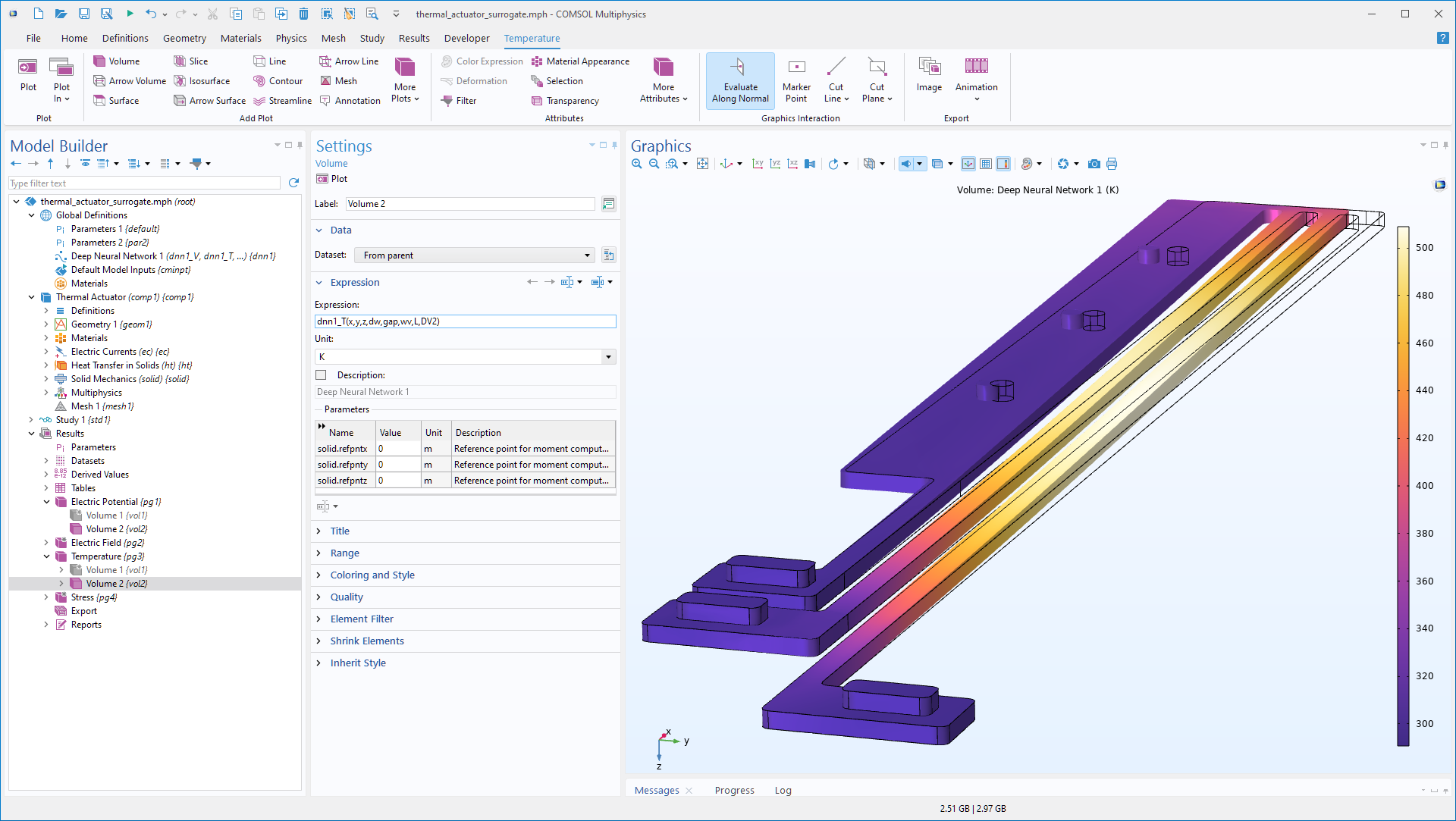
To generate a temperature plot from the surrogate model function, simply call it from theExpressionfield in the plot settings, as shown in the figure below. In this example, the expressiondnn1_T(x,y,z,dw,gap,wv,L,DV2)is used, where the results parameterDV2is specified instead ofDVto accelerate the field plot when the geometry remains unchanged.

The Model Builder with the Volume plot selected under the Temperature plot group node with the corresponding Settings and Graphics windows displayed.

Generating a plot using a call to a surrogate model function.

Similarly, surrogate model function calls can be used for numerical result evaluations. For example, in the app, the maximum temperature is displayed by calling the same function in aVolume Maximumevaluation underDerived Values, as shown in the figure below. A method is used to toggle between the DNN function call and a direct reference to the finite element variableT, depending on whether the full solution is computed and visualized.

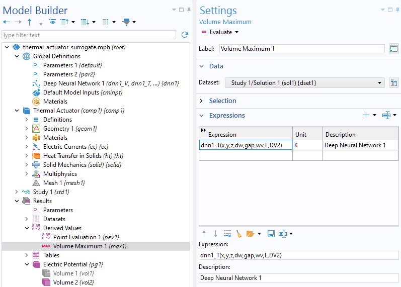
Generating numerical output using a call to a surrogate model function.

Note that spatially varying surrogate model functions, trained on geometry sampling data, need to be evaluated and visualized within the context of the parametric CAD geometry and finite element mesh. Visualizing these surrogate model functions as response surfaces (or volumes) alone would lack the appropriate context, as the extent and boundaries of the geometry are not well defined using a simple Cartesian grid. In this case, the complete surrogate model consists of both the surrogate model function and the finite element mesh on which it was trained.

Efficient Time-Domain Sampling: Battery Test Cycle Surrogate Model App Overview

Similar to efficient geometry sampling, theSurrogate Model Trainingstudy can also be used to generate time-domain, frequency-domain, or parametric data. Efficient time sampling is demonstrated in theBattery Test Cycle app, which is available in the Application Libraries of the Battery Design Module. This app demonstrates the usage of a surrogate model function for predicting the cell voltage, cell open-circuit voltage, and internal resistance of an NMC111/graphite battery cell undergoing a battery test cycle. The DNN surrogate function is fitted to a subset of the possible input data values. Five input data values can be set: the current in four segments of the cycle and the initial state of charge of the battery cell. The low computational cost of evaluating the surrogate function allows knobs to be used to interactively combine the input values and predict the cell voltage and internal resistance. Once a combination of values has been selected, the prediction of the surrogate model can be verified by computing the actual physical Li-ion battery model.

A screenshot of the UI for the surrogate model of a battery test cycle simulation app.

The Battery Test Cycle app demonstrating the use of a DNN surrogate model to reconstruct time-varying physical quantities.

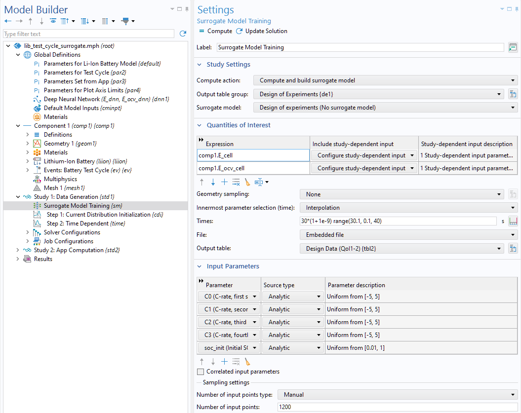
In theSurrogate Model Trainingstudy, the time steps from theTime Dependentstudy are referenced by a vector. Similar to geometry sampling, the entire range of output values corresponding to this time vector is saved in batches to the data file. These settings are shown in the figure below.

The Model Builder with the Surrogate Model Training node selected and the corresponding Settings window.

TheSurrogate Model Trainingstudy settings for efficient time-domain sampling.

The DNN surrogate model includes 6 input features, 2 output features, and 2 hidden layers, with a layer configuration ofandactivation functions, as shown in the figure below. TheData Column Settingssection reflects the quantities of interest and input parameters from theSurrogate Model Trainingstudy, with the last column originating from the time sampling vector. The DNN surrogate model defines 2 DNN functions with 6 input arguments.

The Model Builder with the Deep Neural Network function selected and the corresponding Settings window.

The DNN surrogate model settings with two functions in six input arguments.

The surrogate model reconstructs time-varying data using a method known astime-series stitching. For a detailed explanation of this method, refer to the documentation for the app. Additionally, the sampling method described here can be applied to any parametric data by treating the parameter space similarly to how time data is managed in the Battery Test Cycle app.