学习中心

Creating a Multiphysics-Driven Deep Neural Network Surrogate Model

---

To illustrate the process of creating a surrogate model for a multiphysics simulation and parametric CAD model, we will create a surrogate model for the displacement of a thermal actuator. In this course, we will ultimately develop a surrogate model that captures virtually all aspects of the thermal actuator. For now, we will begin with a basic surrogate model that requires minimal data. Despite its simplicity, this initial physics-based example will help you better understand the process of developing this type of surrogate model in COMSOL Multiphysics^®. Additionally, this example shows a technique for generating a response surface using a deep neural network.

Thermal Actuator Model Overview

Start by loading the thermal actuator tutorial model from the Application Libraries in the software. Multiple versions of the model are available under theCOMSOL Multiphysics>Multiphysicsbranch. Select and open the simplified model version.

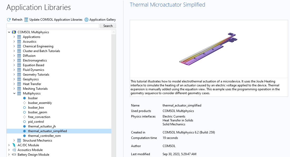A screenshot of the COMSOL Multiphysics UI with the Application Libraries window open and the thermal actuator simplified tutorial model selected, which displays the tutorial model name and an image of the model along with several details and properties regarding the mode.

The thermal actuator tutorial model in the Application Libraries.

Note that this model is also featured extensively, in different variations, in the Learning Center course "Defining Multiphysics Models".

The thermal actuator design includes two hot arms made of polysilicon, as shown in the figure below.

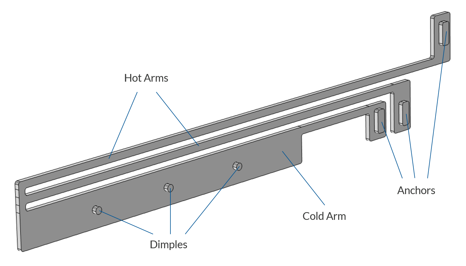
The thermal microactuator geometry with the parts labeled. The device is made of polycrystalline silicon.

The actuator is activated through thermal expansion. Joule heating (resistive heating) is used to achieve the temperature increase needed to deform the two hot arms and consequently displace the actuator. The greater expansion of the hot arms, compared to the cold arm, causes the actuator to bend. The material properties of polysilicon vary with temperature, leading to fully coupled physics. As electric current flows through the hot arms, it raises the actuator's temperature, triggering thermal expansion. At the same time, the electrical conductivity changes with temperature and the current flowing through the hot arms changes accordingly, in turn affecting the heating and the thermal expansion. Actuator operation thus involves three coupled physics phenomena:

1. Electric current conduction
2. Heat conduction with heat generation
3. Structural stresses and strains due to thermal expansion

The operation of the device is also detailed extensively in the course ondefining multiphysics models.

TheParametersnode contains the parameters of the model, including geometric dimensions such as length, width, and the applied voltage, as shown in the figure below. These are the parameters that we can use as a basis for creating surrogate models.

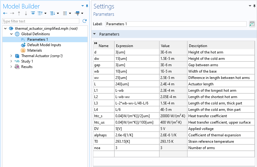The Model Builder with the Parameters 1 node selected and the corresponding Settings window, which contains a tabular list of parameters used in the model.

The parameters driving the thermal actuator model.

Defining the Surrogate Model

Let's now assume that we are interested in creating a surrogate model for predicting the variation in the maximum displacement of the tip of the actuator. Furthermore, assume that we vary just two of the model parameters: the actuator length and the applied voltage, according to the following table:

Parameter	Min Value	Max Value	Unit	Variable Name
Actuator length	150	400
Applied voltage	0.5	10

As output quantity, we have the maximum displacement at the tip:

Quantity of Interest	Type	Unit	Surrogate Model Function Name
Maximum displacement	Scalar

Abstractly speaking, we are defining one surrogate model function:

whereandare the input parameters, representing the length and applied voltage, respectively, andis the maximum displacement at the tip.

The Surrogate Model Training Study

In theory, we could perform a parametric sweep over both input parameters to generate a densely sampled dataset in this simple case. However, in many practical scenarios, this approach is computationally prohibitive. Instead, the parameter space is typically sampled sparsely, requiring surrogate models to accurately approximate unsampled values. This is the reason for using design of experiments (DOE) methods in the data generation process for data-driven surrogate models. DOE methods efficiently explore the parameter space, capturing the essential variations necessary for accurate model approximation. We will begin the process of creating a surrogate model by using aSurrogate Model Trainingstudy, which will take care of the DOE sampling for us.

To begin with this study, right-click theStudynode and selectSurrogate Model Training.

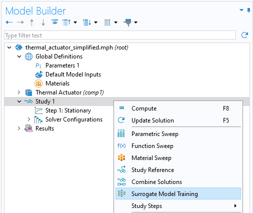
Adding theSurrogate Model Trainingstudy.

TheSurrogate Model Trainingstudy has a number of settings, and the first one we will pay attention to is theQuantities of Interest.

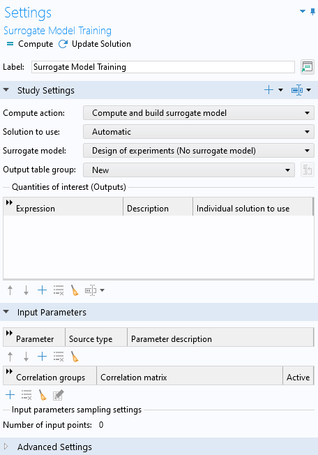
TheSurrogate Model TrainingstudySettingswindow.

We want to provide the maximum displacement as the single quantity of interest. However, we haven't yet created a variable that we can use for this purpose. We will do so through the use of aPoint Probe. Right-click theDefinitionsnode, and underProbes, choosePoint Probe.

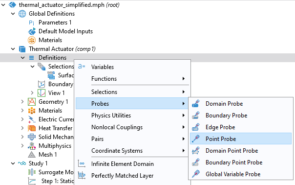
SelectingPoint Probefor accessing the maximum displacement at a point.

In the settings for thePoint Probenode, underSource Selection, selectTip. This named selection is already defined in the Application Library model that we loaded. It contains a selection of a point at the tip of the actuator.

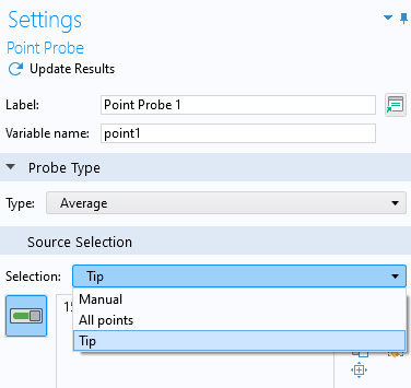
TheSource Selectionfor thePoint Probefeature.

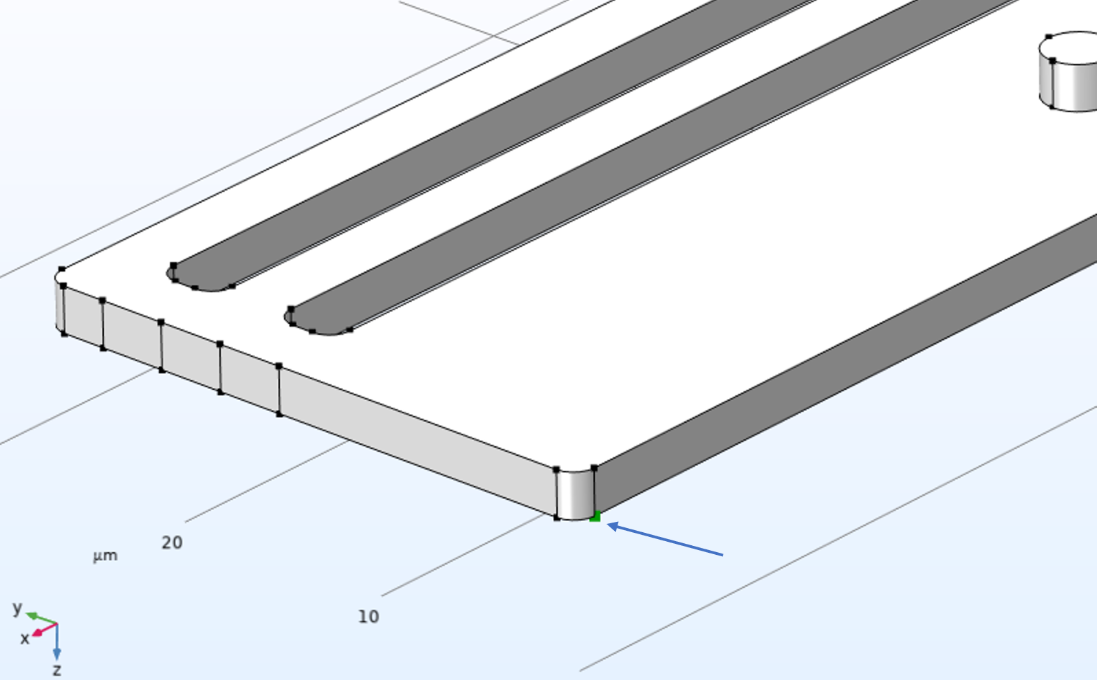A close-up of the thermal microactuator geometry where the point selected for the Point Probe feature displays a green color with an arrow pointing to it.

The location of the point probe where the maximum displacement is measured.

The default expression that is monitored by the probe is the voltage,V. We will now change this to the magnitude of the displacement. Use theReplace Expressionbutton and menu to locate the expression forSolid Mechanics>Displacement>Displacement magnitude, or entersolid.dispin theExpressionfield.

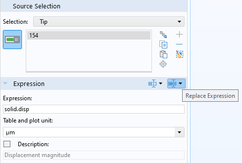
The displacement expression used for thePoint Probe.

You may notice that theTypesetting of thePoint ProbeisAverage. You can also chooseMaximum,Minimum, orIntegral. However for aPoint Probe, they all generate the same result (the average of the value at a point is the value at that point, etc.).

Next, in theSurrogate Model TrainingnodeSettingswindow, click theAddbutton to add a row to the table forQuantities of interest. Then, typecomp1.point1for the value of thePoint Probebelonging to the componentcomp1.

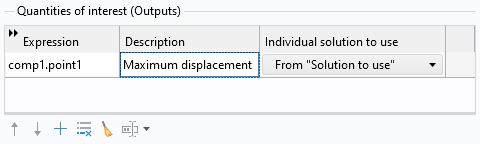
ThePoint Probeused as the quantity of interest.

Alternatively, you canuse Ctrl+Space in theExpressionfield to autocomplete entering the expressionand browse to thePoint Probe, as shown in the figure below.

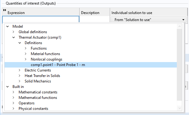
Browsing to the expression for thePoint Probeusing code completion.

We are now ready to specify the parameters to vary in theInput Parameterssection. Use theAddbutton in theInput Parameterstable to add the parametersL (Actuator length)andDV (Applied voltage). For the parameterL (Actuator length), set150for theLower boundand400for theUpper bound, with the unitum(for micrometers). For the parameterDV (Applied voltage), set0.5for theLower boundand5for theUpper bound, with the unitV. To set the bounds, you first click on the corresponding row in theInput Parameterstable. This will make the fields forLower bound,Upper bound, andUnitavailable under the table. Make sure that the length unit of the parameter for the actuator length is set toum, corresponding to micrometers.

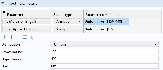
The input parameters settings for theSurrogate Model Trainingstudy.

Before we start generating the data by running the study, we need to define how many data points we want. The number of data points is another term for the number of parameter tuples generated by the study by solving the full finite element model (or other numerical methods used for the model at hand). It is defined by theNumber of input pointssetting in theInput parameters samplings settingssection. Change this setting from the default20to50. This will solve for 50 parameter value tuples for the length and applied voltage with values determined by the underlying DOE method.

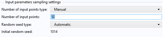
TheNumber of input pointssetting, which determines the number of times the model is solved.

Now it is time to run the computation, which will solve the model 50 times. Right-click theStudynode and selectCompute. The computation will take about 5 minutes on a standard workstation.

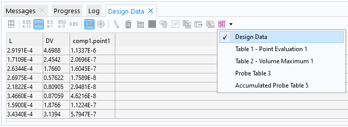
Information on the data generation is displayed in anAccumulated Probe Tableas well as aDesign Datatable, as shown below.

A screenshot of the Messages/Progress/Log window section of the COMSOL Multiphysics UI with the Data Design table displayed.

TheDesign Datatable showing the generated data points.

Note that during the computation you can switch between different tables by selecting from theDisplaymenu button in theTablewindow toolbar. When the computation is finished, theDesign Datatable contains the data we need to train a surrogate model. Note that theSurrogate Model Trainingstudy gives you the option to define an empty surrogate model automatically after the computation. However, the default is to define it manually. This is controlled by theSurrogate modelsettingDesign of experiments (No surrogate model). In this example, we will not change this setting but will define the surrogate model manually.

The generated table data only supports the base unit system, which is the SI unit system in this case. We will need to compensate for this later on when we train the surrogate model.

Building the Surrogate Model

To add the surrogate model, right-click theGlobal Definitionsnode and underFunctionsselectDeep Neural Network.

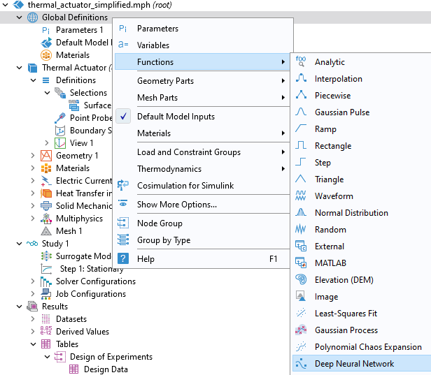
Selecting theDeep Neural Networkoption.

For this surrogate model we can get by with a very small network. Use theAddbutton under the table to create anetwork, according to the figure below. For theData source, selectResults tableand chooseDesign Dataas theResults table. As described in Part 2, the last layer'sOutput featuressetting doesn't need to be changed but is implicitly defined by the number of outputs, or quantities of interest, which in this case is 1, the maximum displacement.

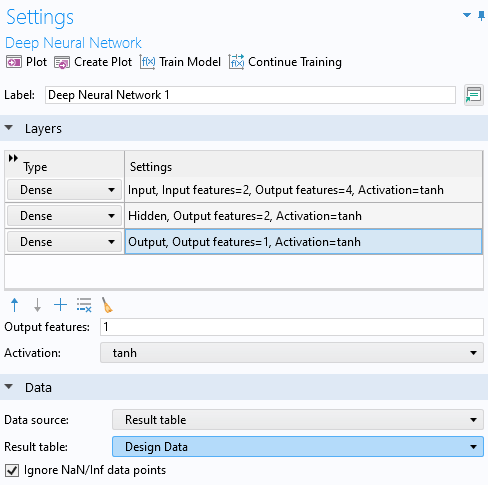
The DNN layer architecture.

Since theDesign Datatable uses the centralized unit system, in this case SI units (m and V), we will define these units in theData Column Settings, as shown in the figure below.

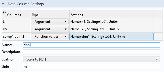
Defining SI units for the surrogate model.

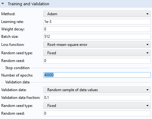
In theTraining and Validationsection, change theNumber of epochsto40,000and clickTrain Modelat the top of theDeep Neural Networkwindow to start the training. TheNumber of epochsvalue is decided by trial-and-error starting from the default value of 1000.

TheTraining and Validationsettings.

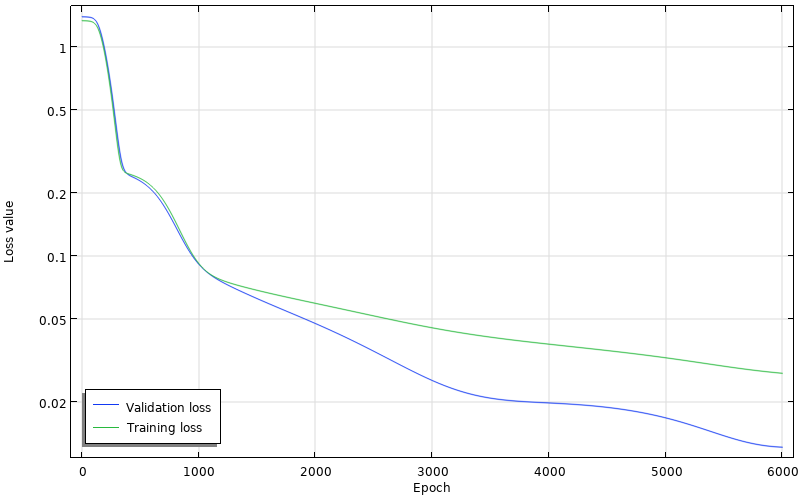
The convergence plot for the DNN training showing the loss for the first 6000 epochs.

The training process is quick in this case since the network is very small. After about 38,000 epochs we see a tendency toward overfitting, so anywhere around this point is a good place to stop the training. Recall that we can identify when overfitting sets in by the fact that the training loss keeps decreasing while the validation loss starts increasing.

A line graph containing a blue line and a green line, which both exhibit erratic spikes and dips in the line, with the epoch number on the x-axis and loss value on the y-axis.

The convergence plot showing the loss for the last epochs.

The lowest value of the validation loss is obtained at about 37,000 epochs, and this is the value that will automatically be used by the surrogate model function.

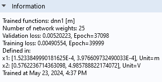
TheInformationsection showing the DNN training results.

We can now plot the surrogate model by selectingCreate Plotin theDeep Neural Networkwindow toolbar.

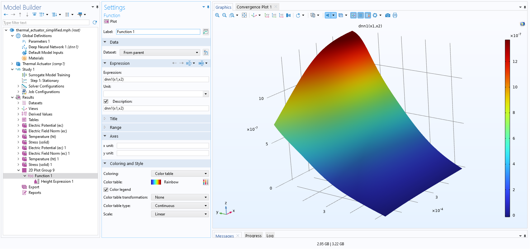The Model Builder with the Function 1 plot node selected and the corresponding Settings window shown and plot visualization displayed.

A visualization of the DNN function.

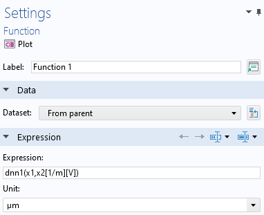
Now, you can change the units for the surrogate model function toµm, as shown in the figure below.

The unit setting for plotting the DNN function.

Note, however, that we cannot change the unit for the x-axis due to the fact that the surrogate model is trained on the data in theDesign Datatable, which is defined in SI units. So, we will keep the unit for the length parameter input argument set to meters.

The DNN function with the height scaled to micrometers.

Comparing the DNN Function with a Linear Interpolation Function

Similar to the example in Part 2, and the fact that we only have two input parameters and one quantity of interest, we can easily visually and quantitatively compare the surrogate model function to an interpolation function.

To perform the comparison, right-clickResultsand add a2D Plot Group. TheDatasetsetting in this plot group now points to aGrid 2Ddataset that was automatically added when we selectedCreate Plotin theDeep Neural NetworknodeSettingswindow. Note that theGrid 2Ddataset only supports length units — meters, in this case — so we need to keep in mind that the axis forx2is a voltage quantity. Due to this limitation, we will keep all unit settings to their defaults.

Right-click the new2D Plot Groupnode and add aSurfaceplot. In theExpressionfield, typednn1(x1,x2)and clickPlot.

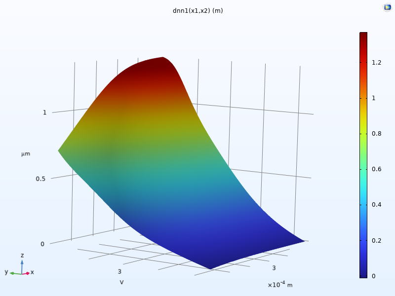
Now, let's add a linear interpolation function to compare with.

Right-click theGlobal Definitionsnode and underFunctionsselectInterpolation. In theInterpolationnodeSettingswindow, change theData sourcetoResult tableand make sure theTable fromsetting is set toDesign Data. Change theNumber of argumentsto2. This will allow the interpolation function to take the length and voltage as input arguments and output the displacement.

The interpolation function based on theDesign Datatable.

In theSettingswindow for the interpolation function, clickCreate Plot.

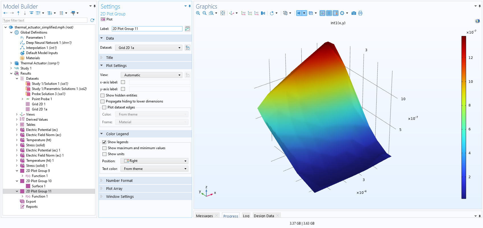"The Model Builder with the 2D Plot Group 11 node selected and the corresponding Settings window and plot displayed in the Graphics window.

A visualization of the table data as a linear interpolation function.

Now, to compare with the DNN function, first navigate toGrid 2D 1. Change theFunctionsetting fromDeep Neural Network 1toAll. This will allow the visualization of any of the functions available underGlobal Definitions.

Next, locate the plot group with theSurfaceplot of the DNN function. In this case, it is2D Plot Group 10. Right-click2D Plot Groupand selectSurface. In theExpressionfield, typeint1(x1,x2). In theSurfacewindow, clickPlot. This will generate two superimposed plots.

In order to separate the plots, we will add aHeight Expressionnode. Right-clickSurface 1and selectHeight Expression. Change theScale factorto1e6.

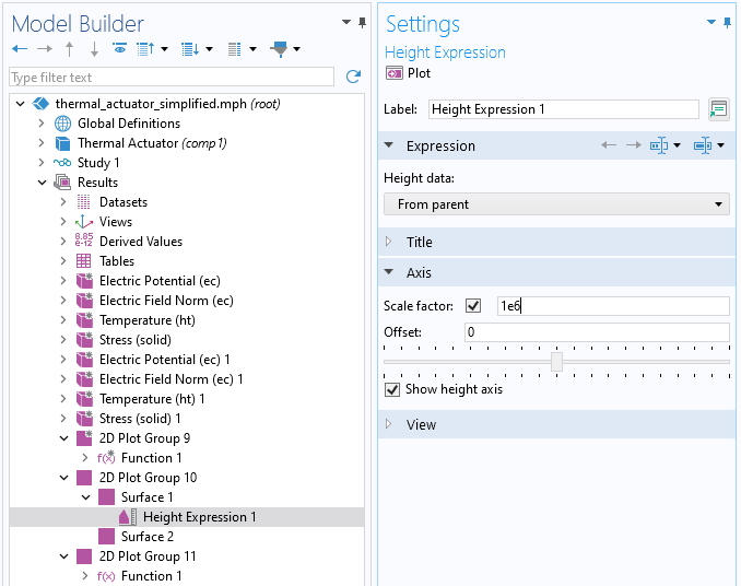
TheScale factorsetting in theSettingswindow for theHeight Expressionnode.

Next, right-clickSurface 2and selectHeight Expression. Change theScale factorto1e6. This gives the two function plots the same height scaling, which enables a proper comparison. InSurface 2>Height Expression>Settingswindow, clear the checkbox forShow height axis. For theColor tablesetting in theSurface 2window, change the option toGrayScale. This produces the result shown in the figure below.

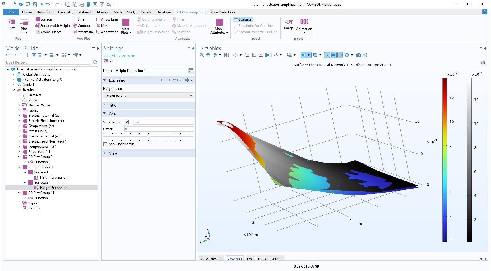The Model Builder with the Height Expression node selected and the corresponding Settings window and plot in the Graphics window. The Graphics window shows a rectangular-shaped surface plot in 3D space that partially displays a rainbow color distribution from dark red to dark blue and partially displays a grayscale color distribution from white to black.

The DNN function plot compared to the corresponding linear interpolation function plot.

We see that the two functions are close in their values. To further analyze their differences, you can evaluate or visualize the expressionabs(dnn1(x1,x2)-int1(x1,x2))using aSurfaceplot in a new plot group. You can try this on your own. In cases where only two input arguments are involved, an alternative approach would be to use a denseParametric Sweepmethod. However, this method becomes increasingly costly for surrogate models with more input arguments, as the computational expense increases with the number of inputs.

In the next part, we will discuss using aGaussian Processsurrogate model, available in the Uncertainty Quantification Module, highlighting the pros and cons of such a surrogate model.