Creating a Gaussian Process Surrogate Model from Imported Data
To learn how to create aGaussian Process(GP) surrogate model from imported data with COMSOL®, we will, for simplicity, use a dataset similar to the example fromPart 2in this article. The data forms a function surface in which the variables
 ,
, , and
, and can represent any quantity such as displacement, stress, temperature, or current. The workflow presented here is applicable when the data originates from experimental results.
Using a GP model, we can create a smooth surrogate model function and associate uncertainty with the fitted data. Additionally, with the Uncertainty Quantification Module, an add-on to the COMSOL Multiphysics®software, we can compute statistical metrics such as the global mean and variance of the surrogate model.
Note: The Uncertainty Quantification Module is required for this example.
Fitting Imported Data with Surrogate Models
The data consists of 900 data points and is stored on a text file format with columns for the arguments and function values. The beginning of the text file, availablehere, appears as follows:
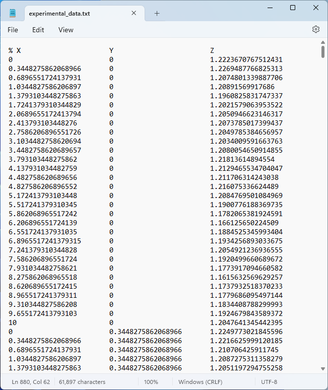
Experimental data in text file format.
We assume that this data represents experimental data. However, in this example we will not be concerned with what the data represents but instead take an abstract approach that is applicable to any type of data. Previously, in Part 2, we learned how to fit experimental data to a linear interpolation function as well as a DNN surrogate model function. Linear interpolation is an efficient method for both 2D and 3D data. However, when creating surrogate models with more than three input arguments, other methods offer significant advantages. Additionally, for noisy data where approximation is needed rather than interpolation, creating a linear interpolation function is often not the best choice. In this article, we will discuss how to use a GP surrogate model to approximate the imported data.
Fitting Imported Data with a Gaussian Process Surrogate Model
Instead of directly importing the data file to a surrogate model function definition, let's start by importing the data file into a table in the software. This makes it easier to reference the same data file from different surrogate models. Start by choosing theBlank Modeloption in the Model Wizard. Then, under theResultsnode, right-click theTablesnode and selectTable.

Adding a table to the results.
In theTablenodeSettingswindow, clickImportand browse to the text file containing the experimental data. This file contains a header beginning with a%character, which is the standard COMSOL format for comments and headers. The columns will automatically be labeledX,Y, andZ.
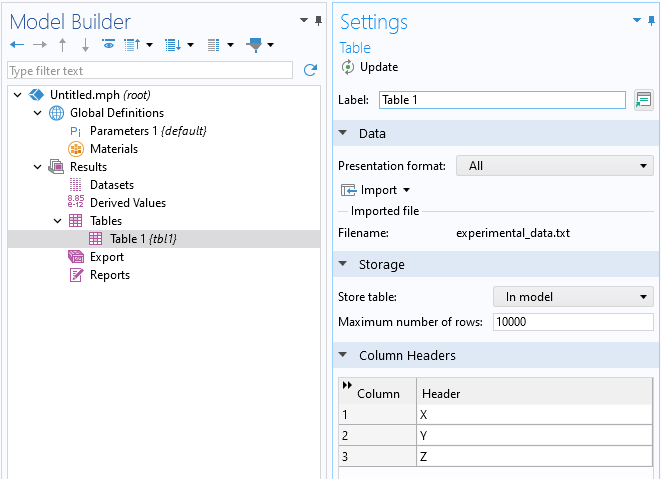
TheTablenodeSettingswindow with the imported data file.
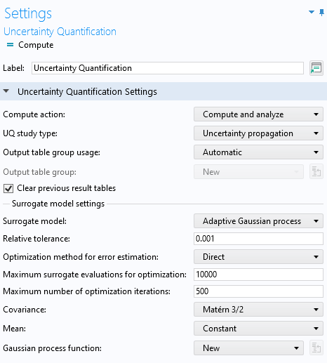
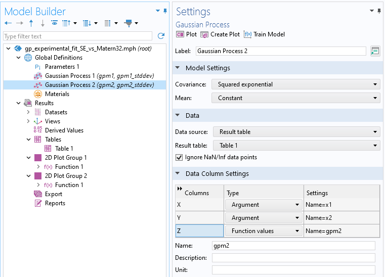
With the Uncertainty Quantification Module, you can now add aGaussian Processsurrogate model function. To do this, right-clickGlobal Definitions, and from theFunctionsmenu selectGaussian Process.
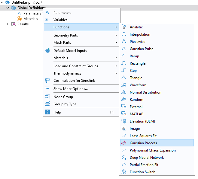
Adding aGaussian Processsurrogate model.
In theGaussian ProcessfunctionSettingswindow, for theData sourcechooseResults tableand selectTable 1. TheData Column Settingssection will automatically be filled out with defaultArgumentandFunction values:x1,x2, andgpm1.
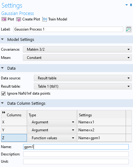
The settings for the GP surrogate model.
In order to assess the uncertainty in the model, we can compute the estimated standard deviation at each point in the dataset. To do this, in theGaussian ProcessfunctionSettingswindow, under theRelated Functionssection, selectDefine standard deviation function. This makes a function namedgpm1_stddevavailable, which can be visualized and evaluated just like any other function.
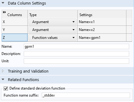
Enabling the standard deviation function,gpm1_stddev,for the GP function,gpm1.
To generate the surrogate model, clickTrain Modelat the top of theGaussian ProcessfunctionSettingswindow. The computation will take a minute or two. Once it is complete, plot the function by clicking theCreate Plotbutton, as shown in the figure below.
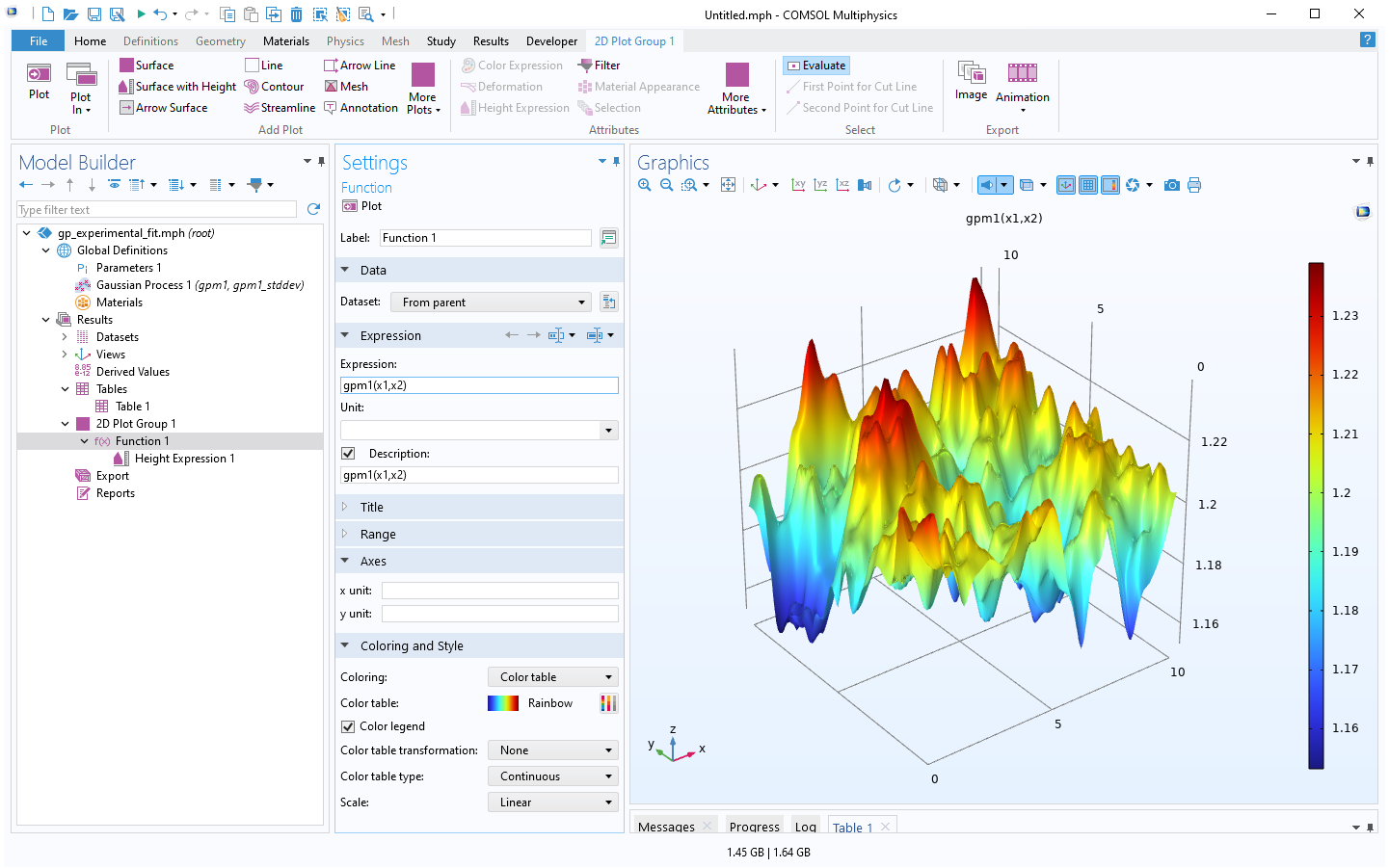 The Model Builder with the Function 1 node selected under 2D Plot Group 1 and the corresponding Settings window and Graphics window.
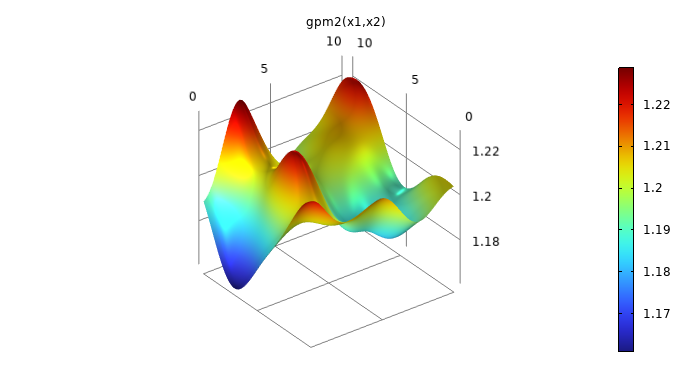
A visualization of the GP surrogate model created from experimental data.
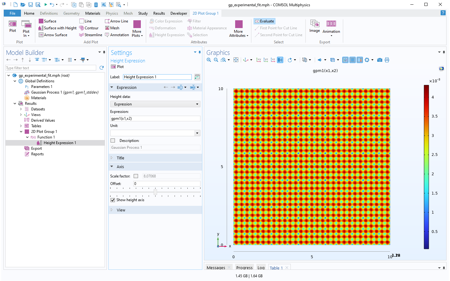
The dataset appears to vary wildly. However, this is due to the automatic z-axis scaling, and upon further inspection, the function values are within a narrow range between about 1.15 and 1.24. We are now interested in computing the pointwise uncertainty in terms of standard deviation as well as the global mean value and standard deviation. Let's start with the pointwise uncertainty. Navigate to theHeight datasetting under theHeight Expressionsubnode and change it toExpressionand typegpm1(x1,x2).
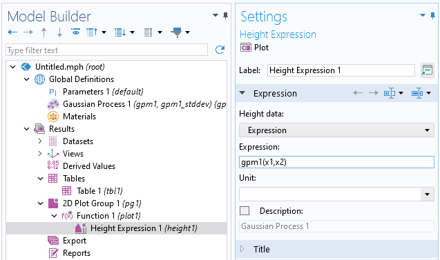
The modifiedHeight Expressionsubnode settings.
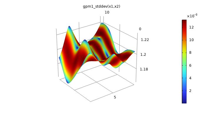
Now, go to theFunctionnodeSettingswindow under the2D Plot Groupnode and change theExpressiontogpm1_stddev(x1,x2)and clickPlot. This generates a visualization of the pointwise standard deviation as a color, as shown in the figure below.
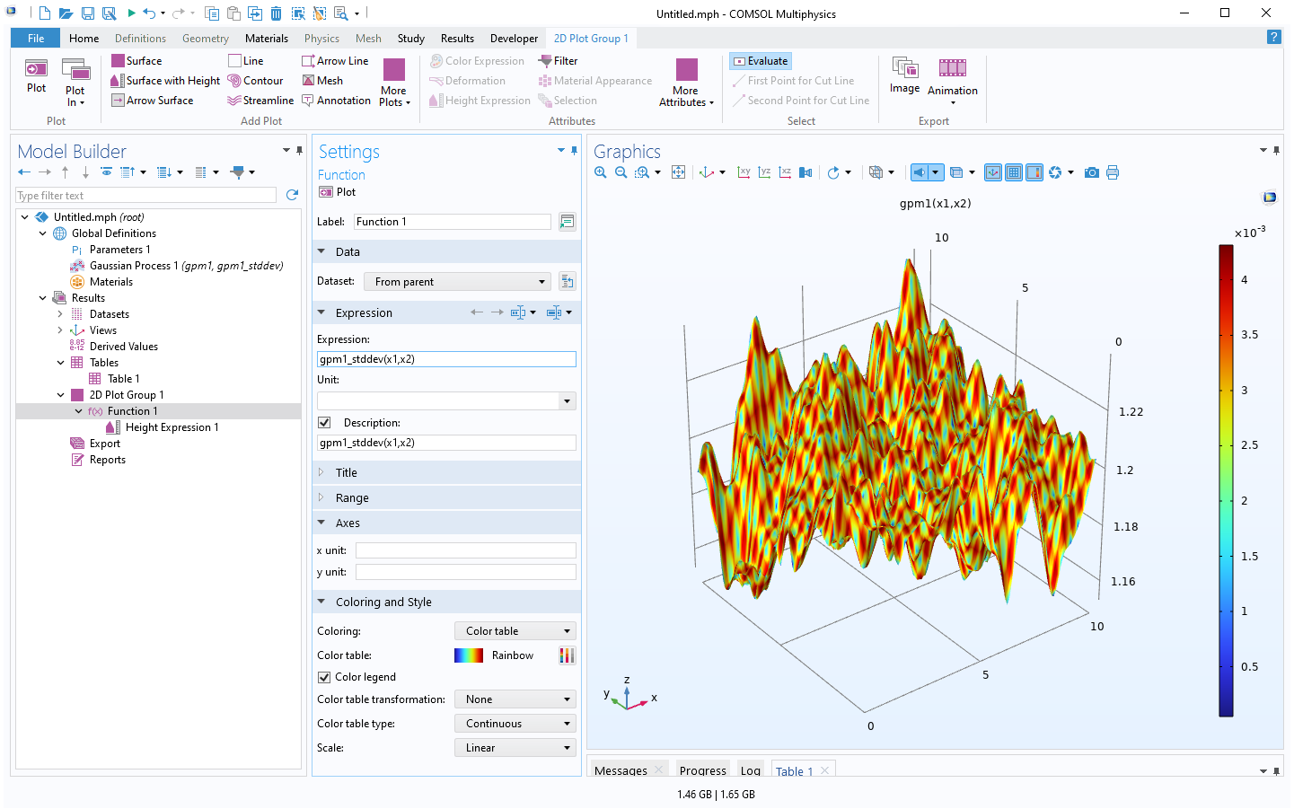 The Model Builder with the Function 1 node selected under 2D Plot Group 1 and the corresponding Settings window and Graphics window.
The standard deviation estimate for the surrogate model.
To better see the uncertainty, we can view the plot in the xy-plane by clicking the xy-button in theGraphicswindow toolbar. Additionally, click theOrthographic Projectionbutton for a better view without perspective effects. You can also optionally click theScene Lightbutton to get a more uniform-looking plot.
 The Model Builder with the Height Expression 1 node selected and the corresponding Settings window and Graphics window.
The standard deviation estimate for the surrogate model, viewed in the xy-plane.
From the standard deviation plot, we can see that the data appears to be sampled in a grid since the standard deviation values are near or at zero in the vicinity of the data points.
In general, a few different factors affect the estimated standard deviation values:
- Distance from training points: Points far from the original data points tend to have higher uncertainty because the model has less information to base its predictions on. This includes extrapolated regions.
- Data density: Areas with sparse data points will generally have higher uncertainty.
- Model complexity and noise: The chosen covariance function (kernel) and noise level in the GP model can also affect the uncertainty. More complex models with more noise might show higher uncertainty.
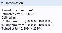
In theInformationsection, at the bottom of theGaussian ProcessfunctionSettingswindow, you can see the globalEstimated errorfor the surrogate model function fit. This value is scaled relative to the standard deviation of the training data (sample standard deviation). In a case where there are multiple quantities of interest and corresponding functions, there is one estimated error value for each function.
TheInformationsection.
Computing Uncertainty with the Uncertainty Quantification Study
The standard deviation indicates a pointwise error boundary around the predicted values. The pointwise mean function is the surrogate model function itself. The Uncertainty Quantification Module includes a solver option that enables computing the global mean and standard deviation of the surrogate model, alongside with some other statistical quantities. Let's see how to use this solver option, building on the previous example. Right-click the root node in the model tree and selectAdd Study. Alternatively, in the ribbon, click theStudytab and selectAdd Study.
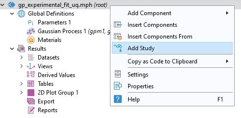
Adding a study.
In theAdd Studywindow, selectStationaryand then close theAdd Studywindow. Now, right-clickStudy 1and selectUncertainty Quantification>Uncertainty Quantification.
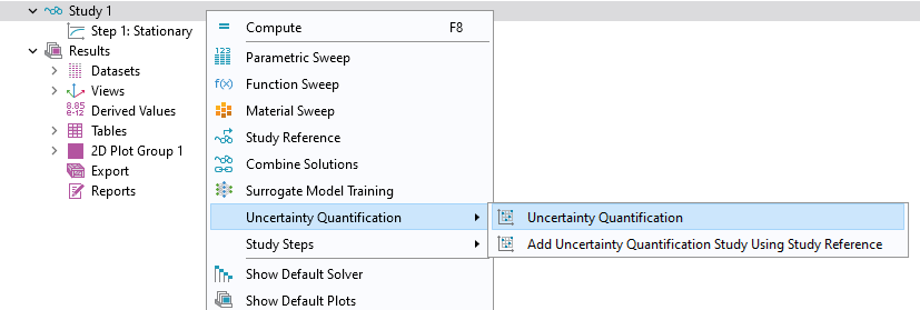
Adding anUncertainty Quantificationstudy.
TheUncertainty Quantificationstudy requires defining quantities of interest and input parameters. Of the five different study type options offered by theUncertainty Quantification Study, we will select the one calledUncertainty propagationfrom theUQ study typemenu. To learn more about these study types, see our course onuncertainty quantification.
TheUncertainty Quantificationstudy settings with theUncertainty propagationoption selected.
Make sure that you have selected theUncertainty propagationoption. In theSurrogate model settingssection, selectGaussian Process 1for theGaussian process function.
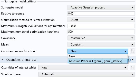
Selecting an already existing GP surrogate model in the uncertainty propagation study.
Change theCompute actionsetting from the defaultCompute and analyzeoption to theAnalyze onlyoption. TheAnalyze onlyoption will use the already-trained surrogate model function for the analysis. Note that the other settings in theSurrogate model settingssection of theUncertainty QuantificationstudySettingswindow only applies when we choose theNewoption for theGaussian process functionsetting.
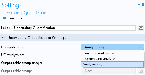
SelectingAnalyze onlyas theCompute action.
The default surrogate model for uncertainty propagation isAdaptive Gaussian process. However, in this case, we will reuse an existing surrogate model, so the adaptive method will not be invoked. The adaptive method requires the generation of new data points, which is not possible for imported data since there is no finite element model to compute additional data points. Therefore, when we select theAnalyze onlyoption, the adaptive method is automatically disengaged, and there is no need to change this setting.
The available surrogate model options are:Adaptive Gaussian process(demonstrated in Part 4),Gaussian process,Adaptive sparse polynomial chaos expansion, andSparse polynomial chaos expansion, as shown in the figure below. In this example, both theAdaptive Gaussian processand theGaussian processoptions use a nonadaptive Gaussian process method.
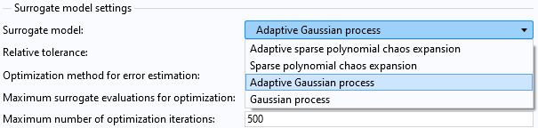
TheSurrogate modeloption in theUncertainty Quantificationstudy.
We will need to create two global parameters that will define the input arguments for the already trained surrogate model so that it can be used by theUncertainty Quantificationstudy. UnderGlobal Definitions>Parameters, create two variables,x1andx2, as shown in the figure below. The actual values are not going to be used but will be overwritten by theUncertainty Quantificationstudy.

The two input argument variables for the surrogate model.
In the case of an already trained surrogate model in combination with theAnalyze onlyoption, we can use anyExpressionfor theQuantities of Interest. Enter1in theExpressionfield forQuantities of Interest, as shown in the figure below. The imported dataset is defined in the region . TheDistributionsetting is set toUniformfor both parameters, which is the only option that makes sense in this example, where we would like to analyze a surrogate model that can be used equally well in any part of the parameter space. In theInput Parameterssection, addx1andx2to the table with a lower bound of0and an upper bound of10for both parameters.
For an already trained surrogate model combined with theAnalyze onlyoption, we can use any expression for the quantities of interest. Enter1in theExpressionfield forQuantities of Interest, as shown in the figure below. The imported dataset is defined in the region. Set theDistributionsetting toUniformfor both parameters, which is the only appropriate option in this example, as we want to analyze a surrogate model that can be applied uniformly across the entire parameter space. In theInput Parameterssection, addx1andx2to the table with a lower bound of0and an upper bound of10for both parameters.

The settings in theQuantities of InterestandInput Parameterssections.
Now we are ready to analyze the surrogate model. At the top of theUncertainty QuantificationstudySettingswindow, clickCompute. Recall that in the case of anUncertainty Quantificationstudy, the sampled variables are output to aQuantities of Interesttable rather than aDesign Datatable.
When the computation is finished, a kernel density estimation (KDE) plot is shown. The KDE plot is a smoothed histogram plot and represents the probability density function estimate for the function value considering all input values in the region. In other words, the KDE plot shows the most probable function values when the input parameter space is randomly uniformly sampled within the set parameter boundaries.
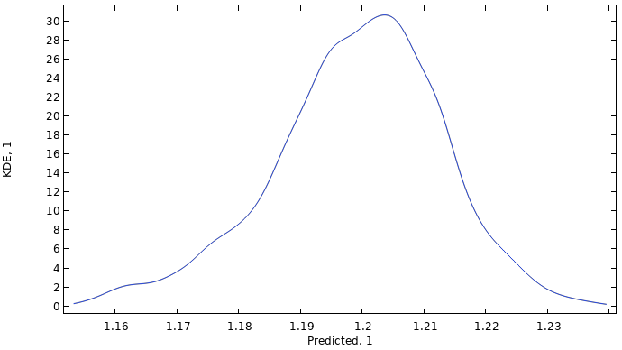
A KDE plot showing the probability density function estimate for the function values of the imported data.
We can also get statistical information from this computation. If not already visible, selectResults>Tables>Uncertainty Propagation>QoI Confidence Interval.
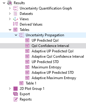
Selecting theQoI Confidence Intervaltable.
TheQoI Confidence Intervaltable contains information about the surrogate model's global mean and standard deviation as well as minimum, maximum, and various quantile values.

TheQoI Confidence Intervaltable.
The global mean value is computed to about 1.2, and the standard deviation is about 0.014, indicating a near constant dataset. The minimum and maximum values are about 1.15 and 1.24, respectively. Note that these values do not correspond to the original dataset but instead to the fitted surrogate model function.
Using Different Covariance Functions
Let's now briefly consider the influence of covariance functions, or kernels. To illustrate this, we will use a more coarsely sampled dataset with only 25 data points compared to the original 900. The figure below shows an example where we have added a second GP function and changed the covariance setting to theSquared exponentialcovariance function. This covariance function is smoother than the default Matérn 3/2 option, as it assumes that the sampled data comes from an infinitely differentiable function. For more information on covariance functions, please refer tothis article.
AGaussian Processsurrogate model using aSquared exponentialcovariance function.
The visualizations below show plots of the surrogate model functions using the Matérn 3/2 and the squared exponential covariance functions. The function based on theMatérn 3/2option appears slightly more "pointy" than the one using theSquared exponentialoption. The Matérn 3/2 covariance function assumes that the underlying data is only once differentiable.
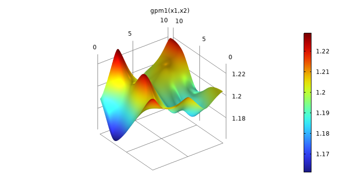 A plot in 3D space of a smooth, curving surface with several hills and valleys and a rainbow color distribution.
 A plot in 3D space of a smooth, curving surface with several hills and valleys and a rainbow color distribution.
Surrogate model functions based on theMatérn 3/2andSquared exponentialcovariance functions.
If we compare the pointwise standard deviation of the two functions, we see that theSquared exponentialcovariance option estimates a lower level of uncertainty. TheMatérn 3/2function provides higher pointwise uncertainty estimates than theSquared exponentialfunction for sparsely sampled datasets because it enables less smooth and more variable functions. This flexibility results in a more cautious model that acknowledges higher uncertainty due to the limited information available, whereas theSquared exponentialfunction, assuming smoother functions, tends to produce lower uncertainty estimates even when data is sparse.
 A plot in 3D space of a smooth, curving surface with several hills and valleys and a rainbow color distribution.
 A plot in 3D space of a smooth, curving surface with several hills and valleys and a rainbow color distribution.
The standard deviation estimates for theMatérn 3/2andSquared exponentialoptions.
Despite the fact that theMatérn 3/2covariance function assumes the underlying data is once differentiable, the computed surrogate model function can be smoother. This is because the surrogate model function represents the mean of the GP posterior distribution, which is derived from all possible GP functions that fit the data, given the Matérn 3/2 covariance. In fact, the mean function is a linear combination of Matérn 3/2 covariance functions. For more information, seethis resourceon covariance functions.
请提交与此页面相关的反馈,或点击此处联系技术支持。